
Solutions of Internal Layers for a Class of Singularly Perturbed Quasilinear Robin Boundary Value Problems with Discontinuous Right-Hand Side
2021-05-26 03:02:06LIUBAVINAlekseiNIMingkangYANGQian
吉林大學(xué)學(xué)報(bào)(理學(xué)版) 2021年3期
LIUBAVIN Aleksei, NI Mingkang, YANG Qian
(School of Mathematical Sciences, East China Normal University, Shanghai 200062, China)
Abstract: We consider a class of singularly perturbed quasilinear differential equation with Robin boundary value conditions and discontinuous right-hand side. Firstly, under the given conditions, the asymptotic expression of a smooth solution with an internal layer in the neighborhood of the discontinuous curve is constructed. Secondly, based on the matching technique, the existence of such solution is proved, and the remainder estimation is given. Finally, the effectiveness of the method is verified by a numerical example.
Keywords: singular perturbation; asymptotic expansion; internal layer; Robin boundary value condition
0 Introduction
This paper studies a piecewise-smooth singularly perturbed quasilinear problem with Robin boundary value conditions

(1)
whereμ>0 is a small parameter,yis an unknown scalar function,A,B,P,Qare some known constants. It’s easy to notice that we can reduce problem (1) to Dirichlet boundary value case if the parameters take certain values.Asymptotic solutions to such problem with Dirichlet boundary value conditions and discontinuity on a vertical line have been investigated by several authors[1-3]. Currently, the main areas where such equations can be used are mechanics and neurology[1-6]. Further researches may lead us to more application fields. One of the key features of such type of task is the existence of an internal layer. It determines a rapid change in a narrow region of the system under consideration. Usually the solution of the problem has internal layers in consequence of large gradients on a given discontinuity line. An example of such situations is studied in the work of reference [7]. In this paper, we have a discontinuity on a monotone curve with respect to the time variable instead of a line. It makes determination of the transition point a bit more difficult task. Discontinuity of this type has appeared in several recent works. An effective method for classical problems with internal layer is presented in the works of references [8-9].
Firstly, we need to formulate the basic conditions for the problem. We require functionsf(t,y),g(t,y) to be sufficiently smooth on the set


Therefore, in the future we will build solutions in these areas. Next let us formulate the basic conditions for constructing an asymptotic approximation.
Condition 1Suppose that the following inequality is true:
ψ(-)(t)>ψ(+)(t),t∈(a,b),
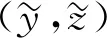
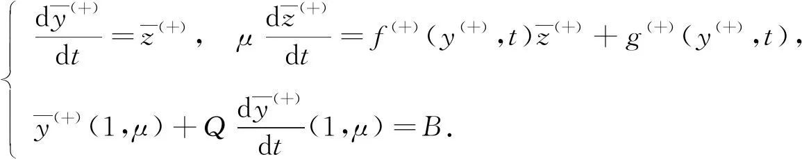
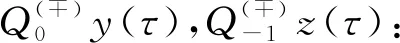
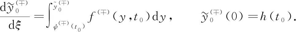
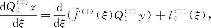
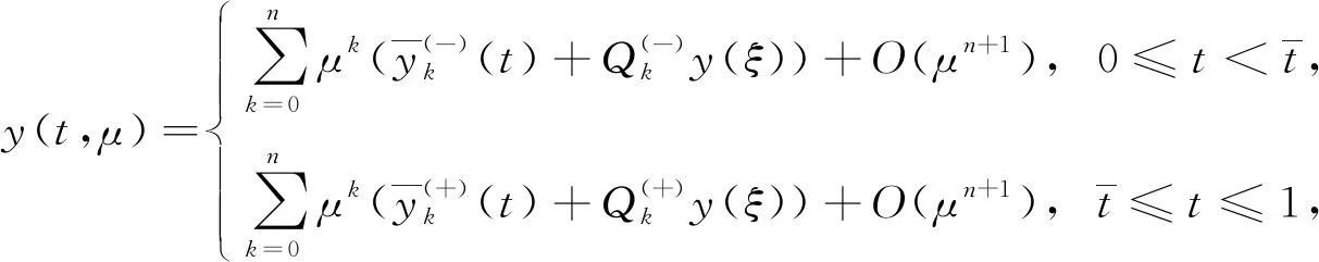
wheret=aandt=bare the abscissas of the intersection points of the curvesy=ψ(±)(t) andy=h(t) respectively. So we can conclude that 0≤a Condition 2Assume that the functionsf(y,t),g(y,t) are of the forms: In addition, the following inequalities hold: Condition 3Suppose that the degenerate problem has a solutiony=ψ(-)(t) on the subdomainD(-), and has a solutiony=ψ(+)(t) on theD(+). Condition 4Suppose that the following inequalities are true: f(-)(ψ(-)(t),t)>0, 0≤t≤1, f(+)(ψ(+)(t),t)<0, 0≤t≤1. Next let us consider the auxiliary system[8] (2) (3) To find the leading term of transition pointt=t*, the following boundary value problem of the system (2) taken att=t0is considered: (4) whereh(x0)∈[ψ(-)(t0),ψ(+)(t0)]. The last two conditions ensure the existence of a solution to this problem and help us to get a smooth internal layer. Condition 5Suppose that the inequalities hold: Let us introduce a new notation Taking into account all of the above, we can formulate the last condition. Condition 6Suppose that the equationI(t)=0 has a solutiont=t0,t0∈[a,b], and it satisfies the inequalityI′(t0)≠0. As mentioned above, asymptotic approximation of the problem (1) will be constructed within two parts. So we will introduce two boundary value problems on the left and right sides of the monotone curvey=h(t) which have the following forms: (5) and (6) According to the standard algorithm, we can reduce them to the systems of the first-order equations: (7) and (8) For the sake of simplicity, we introduce the following notation z(-)(t*,μ)=z(+)(t*,μ)=z(μ). The valuest*andz(μ) are unknown and will be defined later in the asymptotic forms t*=t0+μt1+…+μktk+…, z(μ)=μ-1z-1+z0+μz1+…+μkzk+…. According to Vasileva’s method, the solutions of problems (7),(8) can be written in the forms: (9) where (10) (11) (12) (13) (14) and (15) and According to Condition 3 we have solutions: (16) and (17) where (18) (19) Next we have the internal layer parts. First, according to the standard technique, some extra conditions should be introduced Q(?)y(?∞,μ)=0,Q(?)z(?∞,μ)=0. Just like in the previous part, we first need to define the equations for finding the coefficients. The problems for the internal layer partsQ(?)y(τ),Q(?)z(τ) have the following forms: (20) For clarity of the formulas, we introduce the notation So the problems (20) can be rewritten in the forms (21) From the equations (3), we get (22) (23) It is easy to see that there exist some solutions to these problems, which we can find by basic calculations. where By using basic transformations, you can reduce the equations (25) to the form (28) and the solutions can be written as (29) (30) Here, from the first equality, taking into account Condition 6, the coefficientt0can be found, and from the second equality, the value ofz-1is determined. (31) I′(t0)t1=m1, where According to Condition 6, the coefficientt1is uniquely determined by the following expression: From the second part of expression (31), we can definez0as follows By using this algorithm, we can determine the remaining unknown parameterstk(k=2,3,…). As a result, we obtain a smooth asymptotic representation of the problem (1). Thus, the main theorem can be formulated. Theorem 1If Conditions 2—6 are met, then the problem (1) has a smooth solutiony(x,μ), which has the following asymptotic expression: (32) where Proof: Let us assume that t*=tδ∶=t0+μt1+…+μntn+μn+1(tn+1+δ), (33) whereδis a parameter. According to the statements in the works of references [8-9], for Robin boundary value problems (7),(8), there exist smooth solutionsy(?)(t,μ,δ),z(?)(t,μ,δ) and the following asymptotic representations can be applied: (34) where For the last step, we need to show that if a certain valueδin the expansions (33) is chosen, then the following smoothness condition z(-)(xδ,μ)=z(+)(xδ,μ) is satisfied. Next, we proceed according to the standard scheme. Let us introduce a new notation Δ(tδ,μ)=z(-)(tδ,μ)-z(+)(tδ,μ). From the algorithm of constructingxk(k≥0), we have the equality Δ(tδ,μ)=μn(I′(t0)δ+O(μ)). As an example, consider a simple boundary value problem (35) whereh(t)=2t2+3t-2. The equations and Robin boundary value condition for determiningψ(?)(t) are of the forms Thus we find ψ(-)(x)=2t2+1, (y,t)∈D(-); ψ(+)(t)=-3t2, (y,t)∈D(+). Now we write down the equationI(t)=0. In this case, we have From here we can find that the solution ist0=0.483. By simple computation, we can get internal layer parts Accordig to Theorem 1, the problem (35) has a smooth solutiony(t,μ), whose asymptotic representation is Fig.1 Asymptotic solutions for problem (35) with different values of small parameter Fig.2 Zero-order asymptotic and numeric solutions of problem (35) In this article, the singularly perturbed quasilinear differential equation with discontinuous right-hand side is considered. The case with Dirichlet boundary value conditions and discontinuous terms on the right side of differential equation in the case of vertical line is studied in reference [2]. Instead of a straight line, we take a monotone curve. We have adapted the method for the case of Robin boundary conditions. The existence of a smooth solution for this type of problem has been proved.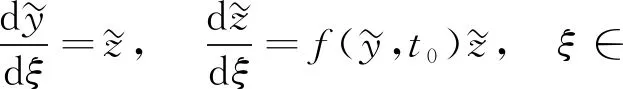


1 Formal asymptotics


1.1 Regular part


1.2 Internal layer functions


1.3 Construction of a smooth solution


2 Main results


3 Example


4 Conclusion
