SHI Yue-yong,CAO Yong-xiu,YU Ji-chang,JIAO Yu-ling

(1.School of Economics and Management,China University of Geosciences,Wuhan 430074,China)

(2.School of Statistics and Mathematics,Zhongnan University of Economics and Law,Wuhan 430073,China)

(3.Center for Resources and Environmental Economic Research,China University of Geosciences,Wuhan 430074,China)

Abstract:In this paper,we consider the variable selection and parameter estimation in high-dimensional linear models.We propose a generalized SELO(GSELO)method for solving the penalized least-squares(PLS)problem.A coordinate descent algorithm coupled with a continuation strategy and high-dimensional BIC on the tuning parameter are used to compute corresponding GSELO-PLS estimators.Simulation studies and a real data analysis show the good performance of the proposed method.

Keywords: continuation strategy;coordinate descent;high-dimensional BIC;local linear approximation;penalized least squares

1 Introduction

Consider the linear regression model

where y∈Rnis a response vector,X ∈Rn×dis a design matrix,β ∈Rdis an unknown sparse coefficient vector of interest and ε ∈ Rnis a noise vector satisfying ε ～ (0,σ2In).We focus on the high-dimensional case d>n.Withou√tloss of generality,we assume that y is centered and the columns of X are centered and n-normalized.To achieve sparsity,we consider the following SELO-penalized least squares(PLS)problem

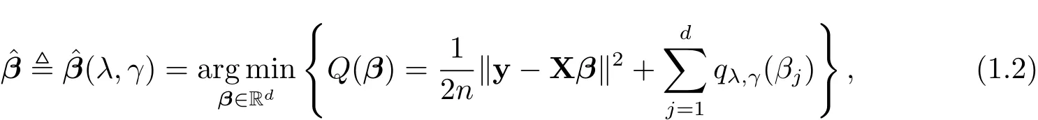
where

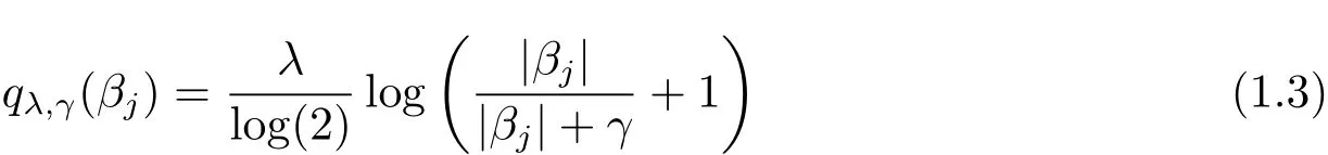
is the SELO penalty proposed by[1],λ and γ are two positive tuning(or regularization)parameters.In particular,λ is the sparsity tuning parameter obtaining sparse solutions and γ is the shape(or concavity)tuning parameter making SELO with small γ values mimic L0,i.e.,qλ,γ(βj)≈ λI(|βj|6=0),when γ is small.

Intuitively,L0penalized methods directly penalize the number of variables in regression models,so they enjoy a nice interpretation of best subset selection[2].The main challenge in implementing L0penalized methods is the discontinuity of the L0penalty function,which results in the lack of stability.As mentioned above,small γ values can make SELO mimic L0,and the SELO penalty function is continuous,so SELO can largely retain the advantages of L0but yield a more stable model than L0.The SELO penalized regression method was demonstrated theoretically and practically to be effective in non convex penalization for variable selection,including but not limited to linear models[1],generalized linear models[3],multivariate panel count data(proportional mean models)[4]and quantile regression[5].

In this paper,we first propose a generalized SELO(GSELO)penalty[6]closely resembling L0and retaining good features of SELO,and then we use the GSELO-PLS procedure to do variable selection and parameter estimation in high-dimensional linear models.Numerically,when coupled with a continuation strategy and a high-dimensional BIC,our proposed method is very accurate and efficient.

An outline for this paper is as follows.In Section 2,we introduce the GSELO method and corresponding GSELO-PLS estimator.In Section 3,we present the algorithm for computing the GSELO-PLS estimator,the standard error formulae for estimated coefficients and the selection of the tuning parameter.The finite sample performance of GSELO-PLS through simulation studies and a real data analysis are also demonstrated in Section 3.We conclude the paper with Section 4.

2 Methodology

Let P denote all GSELO penalties,f is an arbitrary function that satisfies the following two hypotheses:

(H1)f(x)is continuous with respect to x and has the first and second derivative in[0,1];

(H2)f0(x)≥0 for all x in[0,1]and

Then a GSELO penalty qλ,γ(·) ∈ P is given by

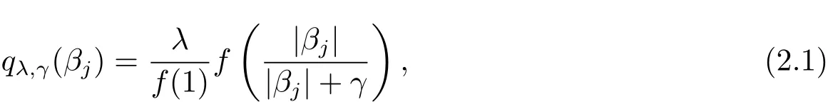
where λ (sparsity)and γ (concavity)are two positive tunning parameters.It is noteworthy that qλ,γ(βj)is the SELO penalty when we take f(x)=log(x+1),and f(x)=x derives the transformed L1penalty[7].Table 1 lists some representatives of P.

Table 1:GSELO penalty functions(LIN,SELO,EXP,SIN and ATN)

The GSELO-PLS estimator for(1.1)is obtained via solving

where qλ,γ(·) ∈ P.

3 Computation

3.1 Algorithm

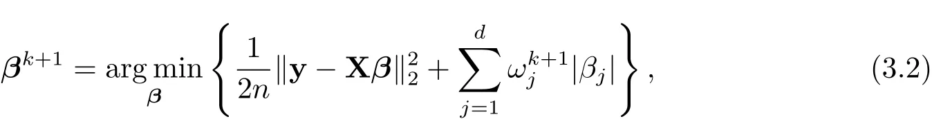
For solving(2.2),we first employ the local linear approximation(LLA)[8]to qλ,γ(·) ∈ P:

3.2 Covariance Estimation

Following[1],we estimate the covariance matrix for?β by using a sandwich formula

?

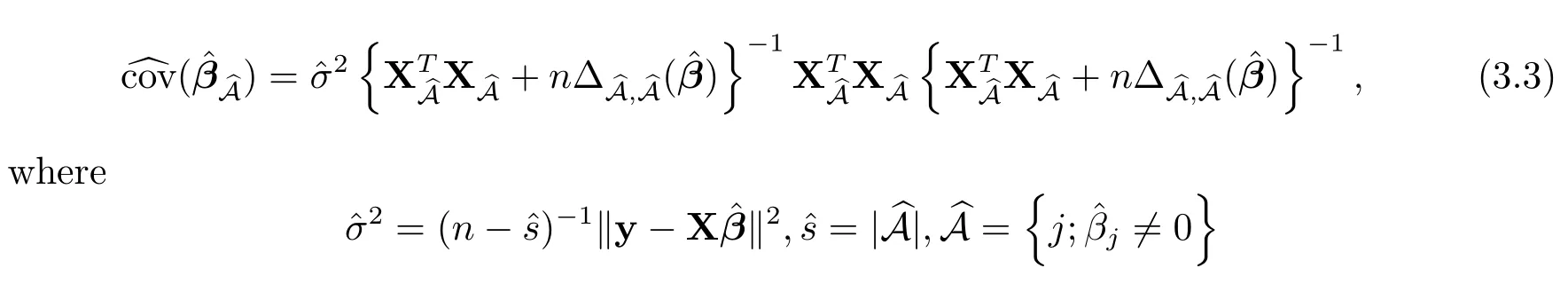
and

For variables with?βj=0,the estimated standard errors are 0.

3.3 Tuning Parameter Selection

Following[1],we fix γ =0.01 and concentrate on tuning λ via a high-dimensional BIC(HBIC)proposed by[10]to select the optimal tuning parameter?λ,which is defined as

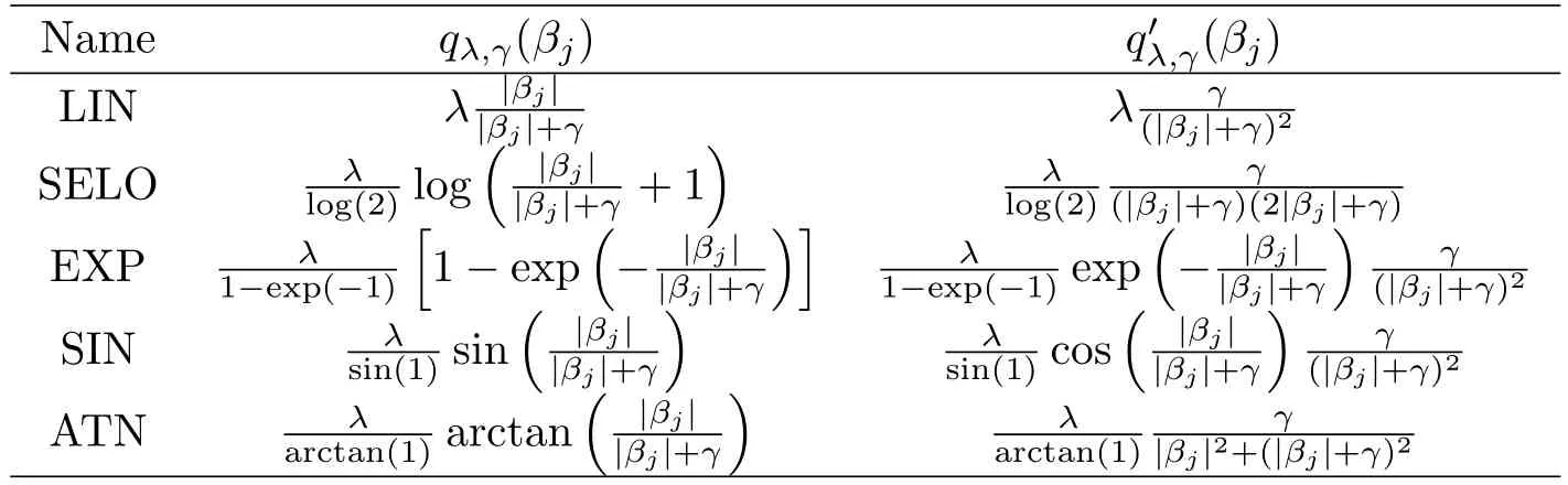
Table 2:Derivatives of GSELO penalty functions(LIN,SELO,EXP,SIN and ATN)

where Λ is a subset of(0,+∞),M(λ)={j:?βj(λ)6=0}and|M(λ)|denotes the cardinality of M(λ),and Cn=log(logn).

For SELO,it is shown in[1]that(λ,γ)=0 for(1.2)whenever λ>λmax,where

Taking qλ,γ(βj)=λI(|βj|0)(i.e.,the L0penalty)in(2.2),we have(λ)=0 wheneverXTy/nk2∞(e.g.,[11]).Since GSELO approaches L0when γ is small,we set λmax=kXTy/nfor GSELO for simplicity and convenience.Then we set λmin=1e ? 10λmaxand divide the interval[λmin,λmax]into G(the number of grid points)equally distributed subintervals in the logarithmic scale.For a given γ,we consider a range of values for λ : λmax= λ0> λ1> ···> λG= λmin,and apply the continuation strategy[11]on the set Λ ={λ1,λ2,···,λG},i.e.,solving the λs+1-problem initialized with the solution of λs-problem,then select the optimal λ from Λ using(3.4).For sufficient resolution of the solution path,G usually takes G≥50(e.g.,G=100 or 200).Due to the continuation strategy,one can set kmax≤5 in Algorithm 1 to get an approximate solution with high accuracy.Interested readers can refer to[11]for more details.

3.4 Simulation

In this subsection,we illustrate the finite sample properties of GSELO-PLS-HBIC with simulation studies.All simulations are conducted using MATLAB codes.

We simulated 100 data sets from(1.1),where β ∈ Rd,with β1=3,β2=1.5,β3= ?2,and βj=0,if j 6=1,2,3.The d covariates z=(z1,···,zd)Tare marginally standard normal with pairwise correlations corr(zj,zk)= ρ|j?k|.We assume moderate correlation between the covariates by taking ρ =0.5.The noise vector ε is generated independently from N(0,σ2In),and two noise levels σ=0.1 and 1 were considered.The sample size and the number of regression coefficients are n=100 and d=400,respectively.The number of simulations is N=100.

To evaluate the model selection performance of GSELO-PLS-HBIC,we record the average estimated model size(MS)the proportion of correct models(CM)the average‘∞absolute error(AE)the average‘2relative error(RE)and the median of the prediction mean squared error(MPMSE)over N simulated datasets,where the prediction mean squared error(PMSE)for each dataset isTable 3 summarizes simulation results for variable selection.With respect to parameter estimation,Table 4 presents the average of estimated nonzero coefficients(Mean),the average of estimated standard error(ESE)and the sample standard deviations(SSD).

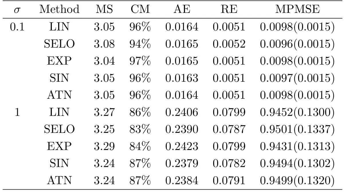
Table 3:Simulation results for model selection.The numbers in parentheses are the corresponding standard deviations of PMSE

Overall,from Table 3 and Table 4,we see that the performance of LIN,SELO,EXP,SIN and ATN are quite similar,and these five GSELO penalties all can work efficiently in all considered criteria.ESEs agree well with SSDs.In addition,all procedures have worse performance in all metrics when the noise level σ increases from 0.1 to 1.

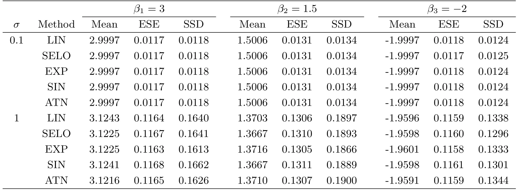
Table 4:Simulation results for parameter estimation

3.5 Application

We analyze the NCI60 microarray data which is publicly available in R package ISLR[12]to illustrate the application of GSELO-PLS-HBIC in high-dimensional settings.The data contains expression levels on 6830 genes from 64 cancer cell lines.More information can be obtained at http://genome-www.stanford.edu/nci60/.Suppose that our goal is to assess the relationship between the firt gene and the rest under model(1.1).Then,the response variable y is a numeric vector of length 64 giving expression level of the first gene,and the design matrix X is a 64×6829 matrix which represents the remaining expression values of 6829 genes.Since the exact solution for the NCI60 data is unknown,we consider an adaptive LASSO(ALASSO)[13]procedure using the glmnet package as the gold standard in comparison with the proposed GSELO-PLS-HBIC method.The following commands complete the main part of the ALASSO computation:

library(ISLR);X=NCI60$data[,-1];y=NCI60$data[,1]

library(glmnet);set.seed(0);fit_ridge=cv.glmnet(X,y,alpha=0)

co_ridge=coef(fit_ridge,s=fit_ridge$lambda.min)[-1]

gamma=1;w=1/abs(co_ridge)^gamma;w=pmin(w,1e10)

set.seed(0);fit_alasso=cv.glmnet(X,y,alpha=1,penalty.factor=w)

co_alasso=coef(fit_alasso,s="lambda.min")

yhat=predict(fit_alasso,s="lambda.min",newx=X,type="response")

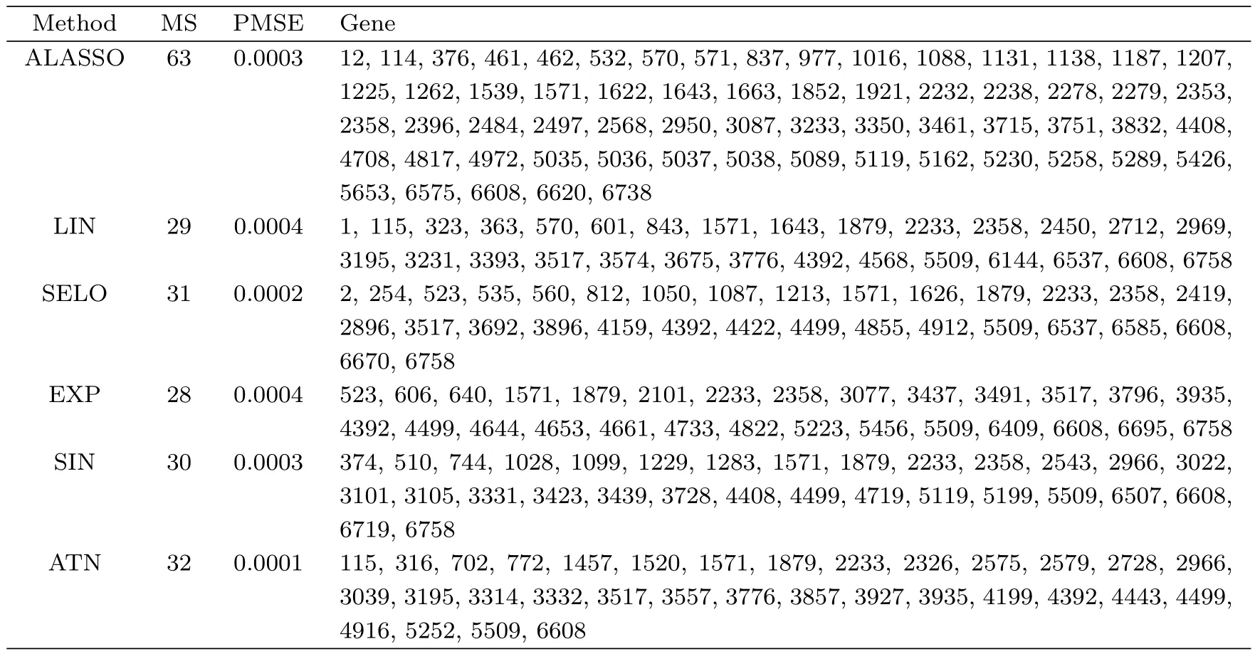
Table 5:Gene selection results of the NCI60 data

Table 6:Estimated coefficients for common genes

Table 5 lists the results of ALASSO and GSELO(LIN,SELO,EXP,SIN and ATN),including the model size(MS),the prediction mean square errors(PMSE)and selected genes(i.e.,the column indices of the design matrix X).From Table 5,six sets identify 63,29,31,28,30 and 32 genes respectively and give similar PMSEs.The results indicate that GSELOPLS-HBIC is well suited to the considered sparse regression problem and can generate a more parsimonious model while keeping almost the same prediction power.In particular,for 2 common genes shown in Table 6,although the magnitudes of estimates are not equal,they have the same signs,which suggests similar biological conclusions.

4 Concluding Remarks

We have focused on the GSELO method in the context of linear regression models.This method can be applied to other models,such as the Cox models,by using arguments as those used in[14,15,16,17],which are left for future research.