Kai Feng(馮凱), Gang Yang(楊剛), and Huichen Zhang(張會臣)

Naval Architecture and Ocean Engineering College,Dalian Maritime University,Dalian 116026,China

Keywords: two-phase flow,lattice Boltzmann method,pressure drop,flow-focusing microchannel

1.Introduction

Gas–liquid two-phase flow in a microchannel is of crucial importance in industrial applications.Extensive studies on the two-phase flow have been conducted.[1–3]

The flow pattern and pressure drop affect the dynamic characteristics of two-phase flow significantly.Different flow patterns can be obtained by controlling the gas–liquid flow rate.[4]Among all the flow patterns, slug flow attracts more attention because of its broad operating conditions and applications.[5,6]The formation of a bubble is under the combined effect of inertia force, viscous force, and surface tension.The capillary number is a vital parameter that affects the generation of bubbles.[7]The length of a bubble can be measured by image observation,which is found to be proportional to the gas–liquid flow rate ratio.The pressure drop gradient can be predicted by correlations based on the homogeneous and separated flow models.[8]To achieve higher prediction accuracy,the two-phase flow pattern should be considered.[9,10]The shear-thinning characteristics of the fluid affect the flow pattern and the pressure drop.The unique flow patterns are observed in the shear-thinning fluid.[11]

Numerical simulation gives information on the flow and pressure fields, which can supplement experimental research and explain the causes of physical phenomena.The lattice Boltzmann method (LBM) has potential applications in multiphase flow simulation because of its advantages of natural parallelism and dealing with complex boundaries.The color gradient[12]and pseudo-potential models[13]are developed to deal with the multiphase flow during the last three decades.Extensive studies have been carried out with these multiphase LBM.However, it is difficult to achieve a large density ratio because of the numerical instability.For a gas–liquid system, the density ratio is 1:800.The phase-field model is a useful tool to deal with the multiphase flow problems, which consists of the classic Navier–Stokes equations and the Cahn–Hilliard or Allen–Cahn equation.[14]With a suitable forcing scheme,the phase-field model can recover the full set of thermohydrodynamic equations for the nonideal fluids[15]and reduce the numerical dispersion.[16]Zhenget al.[17]proposed a phase-field model with a density ratio of 1:1000.In the phase-field model,two distribution functions are employed to calculate the flow field and capture the gas–liquid interface,respectively.It was developed to simulate the impact characteristics of the droplets by Maet al.[18]However,the average gas–liquid density rather than the actual gas–liquid density is used in the model to calculate the Navier–Stokes equation,resulting in a difference in the pressure results with the natural gas–liquid system.Lianget al.[19]developed a new highdensity ratio model with high numerical stability, which can reasonably simulate the gas–liquid system by setting a proper external force distribution function.

The two-phase flow pattern can be captured, while the formation mechanism of the flow pattern is not fully understood.The two-phase pressure drop can be measured on a macroscale and predicted with empirical correlations.However, the mechanism of pressure drop needs to be clarified.The phase-field LBM involving non-Newtonian fluid has not yet been used to simulate the two-phase flow in a flowfocusing junction.This study focuses on the bubble formation and pressure drop in a flow-focusing microchannel.The effects of the gas–liquid flow rate ratio,surface tension,contact angle,and liquid rheological properties are discussed.

2.Number method

2.1.Phase-field LBM

The phase-field LBM improved by Lianget al.[19]is employed to handle the gas–liquid two-phase flow.The distribution functiongi(x,t)is applied to capture the gas–liquid interface,and the evolution equation is given by

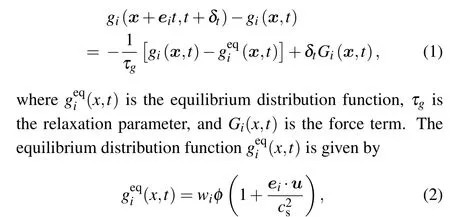
whereuis the fluid velocity,csis the sound speed,wiare the weight factors,w=4/9,w1-4=1/9,w5-8=1/36,andeiare the discrete velocity vectors to neighboring nodes.For a twodimensional nine-velocity model,eiare given by:e=(0,0),ei= (cos[(i-1)π/2], sin[(i-1)π/2)])c, fori= 1–4, andei= (cos[(i-5)π/2+π/4], sin[(i-5)π/2)+π/4])c, fori=5–8,wherecis the lattice speed,c=δx/δt(δxandδtare the lattice spacing and time, respectively).In the phase-field model,φis the order parameter used to distinguish different fluid,which generally takes 1 and 0 in the liquid and gas bulk regions.

The force termGi(x,t)is given by

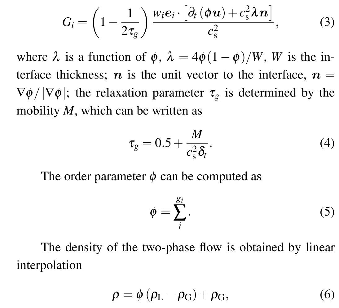
where the subscripts L and G are for liquid and gas phases,respectively.

The distribution functionfi(x,t) is used for solving the flow field,and the evolution equation is written as

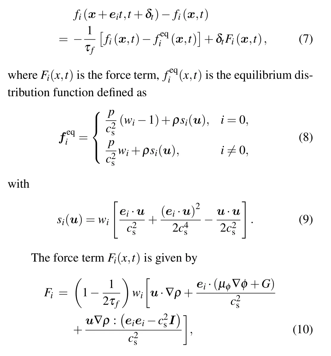
whereGis body force,μφis the chemical potential,which can be calculated as

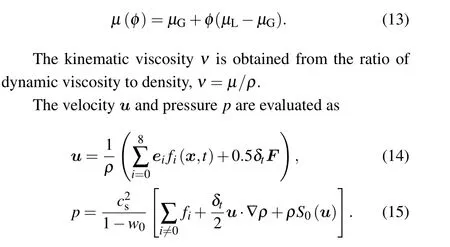
The viscosity of a gas–liquid two-phase system is not a constant value.Linear and inverse linear interpolations of the order parameter were used to determine the viscosity at the interface.[19,20]In present simulation, both the kinematic viscosity and density jump at the interface.To ensure the continuity of the interface, a linear interpolation of the order parameter is used to calculate the dynamic viscosityμof the interface,

2.2.LBM for non-Newtonian fluid

The dynamic viscosity for the non-Newtonian fluid is associated with the shear rate tensor.The simplest and most extensively used power-law model is employed to calculate the viscosity

wherekandnare the consistency coefficient and the flow index,respectively,Dαβis the strain rate tensor.The nonequilibrium part of the distribution function is used to obtain the shear rate tensor,[21,22]and the strain rate tensor can be calculated locally by

where the subscriptsαandβare Cartesian coordinates.

The LBM becomes unstable for small relaxation time,and has poor accuracy for large relaxation time.[20]To achieve higher calculating accuracy and stability,the truncated powerlaw model[23]is adopted to set the range of the lattice kinematic viscosity (0.001≤ν ≤3).The truncated power-law model is given by

The viscosity of a Newtonian fluid is constant.In contrast, the viscosity of a non-Newtonian fluid is not a uniform value.To represent the viscosity of the non-Newtonian fluid,the effective kinematic viscosity (νeff) is employed, which is given by

HereDis the channel diameter,uLis the superficial liquid velocity.

2.3.Wetting boundary condition

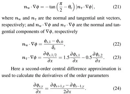
The contact angleθcis used to characterize the wettability of the surface based on Young’s equation,[24]which is calculated as

where the subscript G,L,and S represent the gas,liquid,and solid,respectively.

The schematic of the lattice nodes near the solid wall is shown in Fig.1.

For discussing the three-phase contact line, the lattice nodes near the wall are divided into the fluid layer, solid boundaryy=1/2 and ghost layery=0.[25]According to the geometrical relation, the wetting boundary condition is given by[26]

3.Validation

The two-phase LBM and wetting boundary condition are validated by simulating the water droplets on solid surfaces with different wettability(θc=30?–150?).A circular droplet is initially arranged on the bottom surface.The gas–liquid density ratio and kinematic viscosity ratio are set to 1:800 and 13:1,respectively.To weaken the numerical diffusion,the interface widthAis 5 lattice units.For numerical stability, the mobilityMand kinematic viscosityνare set to:M=0.08,νL=0.1.For simplicity, the density of the gas phase is set to 1.The periodic boundary condition is imposed at the left and right boundaries, while the halfway bounce-back boundary condition is applied to the top and bottom boundaries.The wettability of the solid surface was approached by setting the normal component of the order parameter gradient(see Eqs.(21)–(24)).

The simulation domains are set to 120×48,160×64,and 200×80.The corresponding initial droplet diameters are 36,48, and 60 lattice units, respectively.Numerical simulations are conducted in different simulation domains.The simulation contact angles can be evaluated byθsc=2arctan(2h/L),Landhare the spreading length and the height of the droplet,respectively.[25]The simulation contact anglesθscat different simulation domains are list in Table 1.

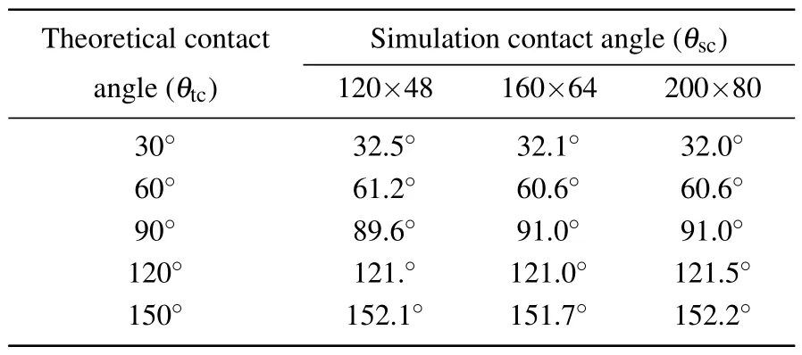
Theoretical contact Simulation contact angle(θsc)angle(θtc) 120×48 160×64 200×80 30? 32.5? 32.1? 32.0?60? 61.2? 60.6? 60.6?90? 89.6? 91.0? 91.0?120? 121.? 121.0? 121.5?150? 152.1? 151.7? 152.2?

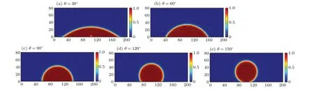
The simulation contact angle varies slightly with the variation of the simulation domain.The simulation contact angles agree with the theoretical values,with a root mean square error of 4.3%, 3.6%, and 3.5% for the simulation domains of 120×48,160×64,and 200×80,respectively.It evidences that the wall contact angle can be well simulated by setting the wall order parameter gradient.In addition, the simulation domain of 200×80 can meet the calculation requirements.The simulation results of water drop shapes with different contact angles at the simulation domain of 200×80 are shown in Fig.2.

In Fig.2,the red part represents a water droplet(φ=1),and the blue part represents the gas phase(φ=0).A dot can be seen in the droplet near the channel wall in Fig.2(a),while it is not a physical phenomenon.The simulation instability occurs in the initial droplet near the three-phase contact line,whenθc=30?.Thus, a small area withφ<1 is observed at the three-phase contact line during calculation.

In our previous study,the truncated power-law model was validated by simulating the Poiseuille flow of the power-law fluids.In addition, it was employed to simulate the vortex characteristics of the non-Newtonian fluid.[27]

4.Results and discussion

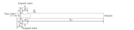
The schematic of the flow-focusing microchannel is shown in Fig.3.The gas phase is introduced from the left inlet,and the liquid phase enters the channel from the top and bottom inlets.The two-phase flow is formed at the junction and exits the channel through the right outlet.

For the physical gas–liquid system, the densities of the gas phase and water are 1.25 kg/m3and 1000 kg/m3, respectively,at the room temperature of 20?C.The gas–liquid density ratio is 1:800.The dynamic viscosities of the gas and liquid phases are 0.0159 mPa·s and 0.97 mPa·s, respectively.[4]The gas–liquid dynamic viscosity ratio is 1:61, and the gas–liquid kinematic viscosity ratio is 13:1 (ν=μ/ρ).In the LBM, the simulation parameters are:ρG= 1,ρL= 800,νL=0.25,νG=3.25,M=0.08,A=5,σ=30.The velocities of the top and bottom liquid inlets are both 0.005.The superficial velocity of the gas inlet is 0.02.The contact angle of the solid wall is set to 90?.The velocity boundary condition is imposed at the inlets.The convective boundary condition is adapted for the outlet.[28]

Firstly,a grid-independence test is conducted.The widths of the microchannel are 30, 40, 50, and 60 lattice units,with corresponding simulation domains of 720×90,960×120,1200×150, and 1440×180.The dimensionless length of the bubble is used to compare the simulation results of different simulation domains,which is the ratio of the bubble length to the channel width.The dimensionless lengths of bubbles in different simulation domains are list in Table 2.

Simulation Width of the Dimensionless width domain microchannel of the bubble 720×90 30 1.3 960×120 40 1.6 1200×150 50 1.58 1440×180 60 1.59

When the simulation domain reaches 1200×150, the dimensionless length of the bubble remains almost unchanged as the simulation domain increases.It indicates that the simulation domain of 150×1200 is suitable for simulating the twophase contact angle problems.The width of the microchannel(D)is 50 lattice units.The lengths of the inlets(L1)are 50 lattice units,and the length of the outlet(L2)is 1100 lattice units.Each lattice space corresponds to 6μm.

Figure 4 shows the two-phase simulation flow pattern and the pressure along the centerline of the microchannel.

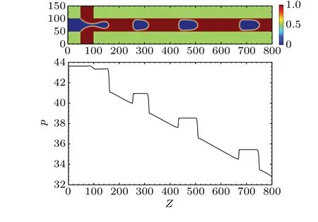
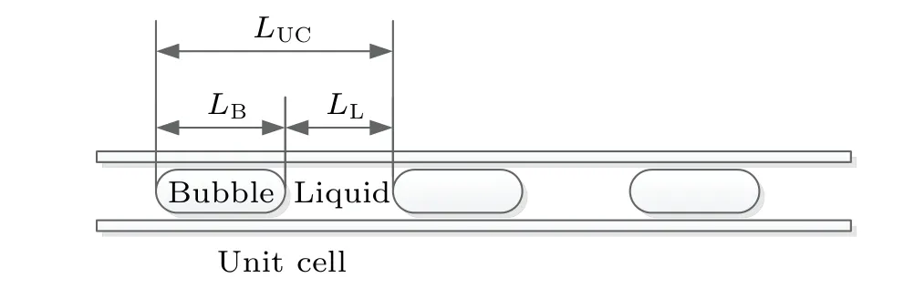
The slug bubbles are formed in the microchannel.In Fig.4, the blue part represents bubbles (φ=0), and the red part represents the liquid phase (φ=1).The liquid film can be seen between the bubble and the channel wall.Corresponding to the two-phase flow pattern,the two-phase pressure drop includes the pressure drop across the bubble and the pressure drop of the liquid slug.The pressure drop gradient of the liquid slug is constant.In the liquid slug,the pressure in front of the bubble is lower than the pressure behind the bubble.This result is consistent with the unit cell model(see Fig.5),which was employed to calculate the pressure drop of two-phase flow with the flow pattern information.[10]

The pressure drop gradient of a unit cell is calculated by

where (dp/dZ)Lis the pressure drop gradient of the liquid slug,pdis the pressure drop across the bubble,LLandLBare the lengths of the liquid slug and bubble,respectively.

The flow rate ratio,surface tension,wetting property,and rheological characteristics of the liquid phase impact the flow pattern and pressure drop significantly.

4.1.Effect of flow rate ratio

The gas–liquid flow rate ratio is a critical parameter in the flow pattern control.The contact angle of the solid wall is set to 90?.At a fixed velocity of the liquid phase 0.01 lattice units,the variation of flow rate ratios is achieved by changing the superficial gas velocity.The range of gas–liquid flow rate ratiocis 1:1–3:1.Figure 6 shows the flow patterns at various flow rate ratios.

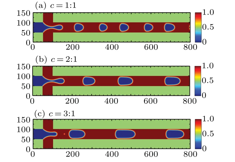
The bubble lengthens with the increase in the flow rate ratio.This agrees with the experimental results.[29]With a small capillary number, the surface tension dominates the viscous force.Thus, bubble generation is mainly controlled by the squeezing regime.The liquid pressure at the junction increases gradually with the liquid flowing into the microchannel from the inlet.When the pressure reaches the cut-off value,the bubble breaks under the squeeze force.The time for reaching the cut-off pressure is constant at a fixed liquid inlet velocity.For a larger flow rate ratio,more gas flows into the forming bubble,resulting in bubble lengthening.

The velocity of the liquid slug increases with the gas velocity, leading to the increase of the pressure drop across the bubble (see Fig.7(a)).The expansion in liquid slug velocity also results in a rise in the pressure drop gradient in the liquid slug.Consequently,the two-phase pressure drop gradient increases with the flow rate ratio,as shown in Fig.7(b).

4.2.Effect of surface tension

The surface tension of the fluid affects the bubble formation significantly.In the simulation, the superficial gas and liquid velocities are 0.02 and 0.01, respectively.The contact angle of the solid wall is set to 90?.The range of surface tension is 20–95.

Figure 8 shows the formation process of a slug bubble atσ=95.The liquid film between the bubbles and the solid wall disappears.This flow pattern is named as the dry-plug flow by Heravi and Torabi.[30]The viscous force is insufficient to make the gas bubble deform.Thus,the forming bubble moves forward, occupying the cross-section of the microchannel after passing through the junction.The liquid accumulates at the intersection,leading to an expansion in the liquid pressure and the break of the forming bubble at the cross-junction.Similar flow patterns are also obtained by Yuet al.[31]and Shiet al.[32]at small capillary number.Similar to the dot in the contact angle simulation,the dots can be seen in the liquid in Fig.8(d).The simulation instability occurs at the gas–liquid interface when the bubble breaks.Therefore, the small areas withφ<1 are observed in the liquid during calculation.

As the surface tension decreases,the capillary number increases, and the slug bubbles are formed in the microchannel atσ=50, as shown in Fig.9.The ratio of viscous force to surface tension increases, causing the deformation of the gas–liquid interface.The liquid film is formed.Therefore,the bubble can no longer occupy the channel’s cross-section after passing through the junction.The squeeze force of the liquid at the cross-junction decreases.The bubble breaks at the right side of the junction under the combined effect of the shear and squeeze forces.

By reducing the surface tension, the capillary number is further increased.Figure 10 shows the bubble formation process in the microchannel atσ=20.front curvature increases.Consequently,the front of the bubble becomes sharper,while the rear becomes blunter with the increase inCa.

For the dry-plug flow,equation(26)is unsuitable for calculatingpddue to the lack of liquid film.The pressure drop across a dry-plug is related to the three-phase contact line and the contact angle hysteresis.[30]Higher surface tension can hold the liquid slug together and reduce the pressure drop across the plug bubble.Consequently, as the surface tension increases,pdfirst increases and then decreases(see Fig.11(a)).

The pressure drop gradient of the liquid slug is related to the fluid velocity and independent of the surface tension (see Fig.11(b)).Thus, the relationship between the pressure drop gradient of the unit cell and the surface tension is consistent with the curve of the pressure difference across a bubble.

With the increase of theCa, the front of the bubble becomes sharper,while the rear becomes blunter.The variation of bubble shape depends on the pressure across the bubblepd,which is related to the surface tension.Thus, the variation of the pressure drop with the surface tension needs to be clarified.The pressure drop across a slug bubblepdincreases with the rise of the surface tension becausepdis positively associated with surface tension,[8]which is expressed as

With the increase inpd, the Laplace pressure across the rear meniscus decreases, while that across the front meniscus increases.Therefore,the rear curvature decreases,and the

4.3.Effect of wetting property

The wetting property of the solid wall is characterized by the contact angle.Different contact angles (θc=30?–150?)can be obtained by adjusting the order parameter near the wall(see Eqs.(21)–(24)).The wettability affects the flow pattern and pressure drop of the two-phase flow by changing the threephase contact line.The superficial gas and liquid velocities are 0.02 and 0.01,respectively.Due to the difference in threephase contact conditions between slug flow and dry-plug flow,the effect of contact angle in these flow patterns are simulated.

Figure 12 shows the flow pattern of slug flow(σ=50)at different contact angles.

The stable slug flow can be seen in the microchannel for all contact angles.No obvious three-phase contact line can be seen because of the liquid film.Thus, the contact angle has little influence on the flow pattern.Becauseθchas little effect on the flow pattern,pdis hardly affected byθc(see Fig.13(a)).Asθcincreases,the drag reduction effect is more pronounced.Thus,(dp/dZ)Ldecreases with the increase inθc.As a result,(dp/dZ)TPdecreases with the increase inθc(see Fig.13(b)).

The dry plug flow is obtained atσ=95.The flow pattern of dry-plug flow under different wall contact angles is shown in Fig.14.

There are apparent contact lines between the gas, liquid,and solid wall.The liquid film cannot be seen anymore.Therefore, the contact angle impacts the flow pattern significantly.With the rise ofθc, the flow pattern of the bubble changed from a convex shape to a concave shape gradually, and the transformation occurred atθc=90?.

The convex curvature of the bubble front is greater than that of the rear.However,the concave curvature of the bubble front is less than the rear.These phenomena can be explained by the pressure of a two-phase flow.The relationship between the pressure across the gas–liquid interface and the curvature is determined by the Laplace formula.For the convex shape flow pattern, the pressure in the bubble is higher than in the liquid.Because of the pressure drop along the microchannel,the pressure in the fluid in front of the bubble is less than the pressure behind the bubble.In comparison,the pressure in the bubble is almost constant.The Laplace pressure at the bubble nose is greater than at the bubble rear,so the convex curvature of the bubble nose is larger than that of the bubble rear.For the concave shape flow pattern, the pressure inside the bubble is lower than that in the liquid.The Laplace pressure at the bubble nose is less than that at the bubble rear.Thus, the concave curvature of the bubble front is less than that of the bubble rear.

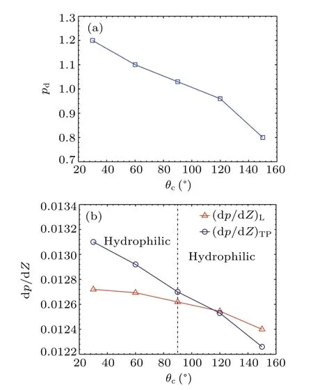
The relationships between the pressure drop gradient in the liquid slug and the pressure drop across a dry-plug bubble with the contact angle are shown in Fig.16.The contact angle hysteresis decreases with the rise inθc.Therefore,the pressure drop across a dry-plug bubble falls withθc(see Fig.15(a)).Because of the drag reduction effect of the hydrophobic surface, (dp/dZ)Ldecreases withθc.Since bothpdand(dp/dZ)Ldecrease with the rise inθc,(dp/dZ)TPdecreases with the increase inθc(see Fig.15(b)).In particular,the pressure drop of the two-phase flow in the hydrophobic surface is slightly less than the pressure drop of the singlephase liquid.

4.4.Effect of non-Newtonian property of the liquid phase

The non-Newtonian property of the liquid plays an essential role in the two-phase flow pattern and pressure drop.Carboxymethyl cellulose (CMC) solution shows shear-thinning characteristics,which is widely used in industry.In the simulation,the CMC solutions with concentrations of 0.1%,0.2%,and 0.3%(CMC 0.1,CMC 0.2,and CMC 0.3)are used.The physical properties of the CMC solutions are listed in Table 3.[4]

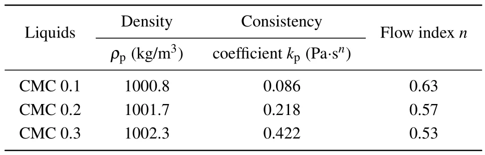
Liquids Density Consistency Flow index n ρp (kg/m3) coefficient kp (Pa·sn)CMC 0.1 1000.8 0.086 0.63 CMC 0.2 1001.7 0.218 0.57 CMC 0.3 1002.3 0.422 0.53

In the simulation, the flow index is set to be the same as the physical properties.However, the consistency coefficient should be set according to the shear rate and the effective viscosity.The effective viscosities of the CMC 0.1, 0.2, and 0.3 can be calculated by Eq.(19).For the superficial liquid velocity of 0.1 m/s, the effective viscosities of the CMC 0.1,0.2, and 0.3 are 4.66, 7.56, and 10.67 mPa·s.The simulation consistency coefficient of CMC solutions with different concentrations are determined according to the viscosity ratios of CMC solutions to water.Thus,the simulation consistency coefficientkof the CMC 0.1,0.2,and 0.3 are 89.33,94.67,and 100.00.The superficial gas and liquid velocities are 0.02 and 0.01,respectively.The contact angles of the solid wall are set as 60?,90?,and 120?.

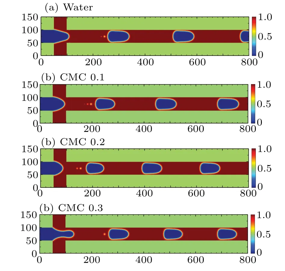
The flow patterns in different fluids atθc=90?are shown in Fig.16.

With increased CMC solution concentration, the bubble front lengthens,and the bubble rear becomes flatter.This phenomenon has also been observed in some experiments,and it is explained to be associated with the shear-thinning characteristics of the liquid phase without detailed discussion.[4,11]In fact, it is related to the capillary number of the fluid.The effective viscosity increases with the increase in the CMC solution concentration, leading to increased capillary number.Therefore, the front of bubble turns sharper and longer, and the rear becomes flatter for a larger capillary number,which is discussed in Subsection 4.2.

The variation of the pressure drop gradient in the liquid slug and the pressure drop across a bubble with the flow index at different contact angles are shown in Fig.17.

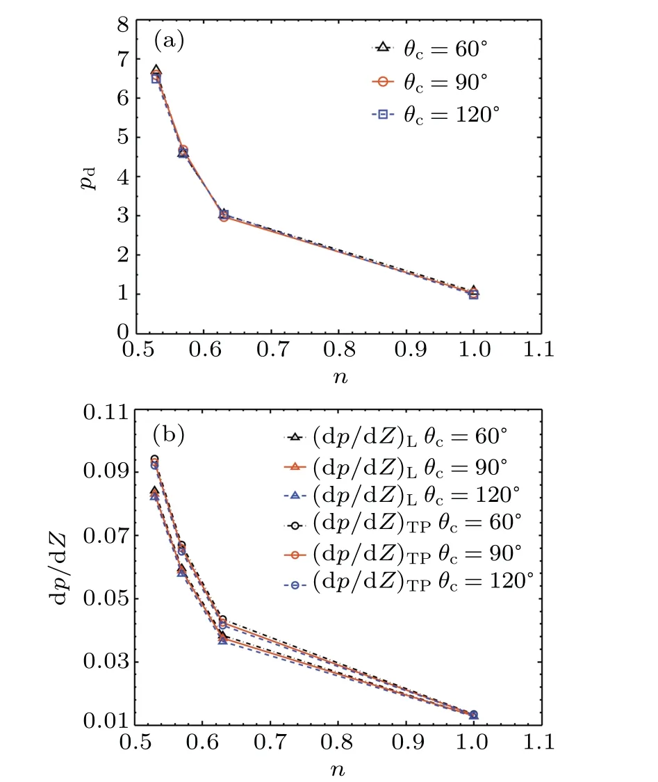
The effective viscosity of the liquid phase decreases with the increase inn, resulting in the reduction ofpdand(dp/dZ)L.Consequently,(dp/dZ)TPdecreases with the flow index.This is consistent with the experimental results.[4]Compared to rheological properties, the effect ofθcon pressure drop is relatively small.Due to the absence of three-phase contact line,the contact angle has almost no effect onpd,and(dp/dZ)Lslightly decreases with the increase inθcbecause of the drag reduction in the hydrophobic surfaces.Therefore,(dp/dZ)TPdecreases with the increase inθcslightly.

5.Conclusion

An LBM for gas–liquid two-phase flow involving non-Newtonian fluid is developed.The two-phase flow pattern and pressure drop are analyzed with this method,considering various parameters, including flow rate ratio, surface tension,wetting property, and rheological characteristics of the liquid phase.The numerical results agree well with the experimental results.

The bubble lengthens with a larger flow rate ratio.The flow pattern transfers from slug flow to dry-plug flow with a sufficiently small capillary number.For the slug flow,θchas little effect on the flow pattern.However,for the dry-plug flow,the front and rear meniscus transfer from convex to concave gradually with the increase inθc.The transformation occurs atθc=90?.The two-phase flow pattern depends on the Laplace pressure across the gas–liquid interface.For the non-Newtonian fluid, the rear of the bubble becomes flatter, and the front becomes sharper for a small flow index,owing to the variation of the capillary number with the flow index.It also shows that the reduced viscosity and increased contact angle are beneficial for the drag reduction of two-phase flow in microchannel.In addition, this work validates the reliability of the developed LBM for simulating the gas–liquid two-phase flow in a microchannel.This method can be utilized to simulate the multiphase problems involving non-Newtonian fluids as well.

Acknowledgement

Project supported by the National Natural Science Foundation of China(Grant No.51775077).