
Dependence of Eigenvalues of Two-Interval Third-Order Boundary Value Problems
2022-01-19 06:24:28LIMenglei李夢磊AOJijun敖繼軍
應(yīng)用數(shù)學(xué) 2022年1期
LI Menglei(李夢磊), AO Jijun(敖繼軍)
(College of Sciences, Inner Mongolia University of Technology, Hohhot 010051, China)
Abstract: In this paper, the dependence of eigenvalues of two-interval third-order differential boundary value problems on various parameters is investigated.Under two types of special boundary conditions, the continuity and differentiability of eigenvalues on the problems are shown, especially the differential expressions with respect to each coefficient functions and boundary conditions are given.
Key words: Two-interval; Third-order boundary value problem; Eigenvalue; Boundary condition; Differential expression
1.Introduction
For the classical Sturm-Liouville (S-L) problems, the solutions of differential equations and their derivatives are continuous in the domain interval, however, such conditions are not always true in some practical problems.Therefore, it is necessary to consider the SL problems with internal discontinuity properties.The differential operator problems with internal discontinuity can be regarded as the studies of differential operators in direct sum spaces.The theory of direct sum spaces also can be seen as the theory of multiple intervals.
For the differential equations on two intervals, in 1986, Everitt and Zettl[1]discussed the self-adjoint theory of second order S-L problems on two intervals under the direct sum in Hilbert spaces.In 2019, WANG[2]studied the self-adjoint domains of odd order differential operators with singular points at both ends of two intervals (the special case is that the endpoint has regular points).The relevant knowledge of the theory of two-interval the readers may refer to [3-4].
The continuity and differentiability of eigenvalues of boundary value problems play an important role in understanding the change trend and the behavior of eigenvalues in theory,so as to calculate the eigenvalues numerically.Therefore, many scholars at home and abroad have carried out a lot of research on the dependence of eigenvalues of second order and even order higher-order differential equations, and have obtained a rich of results[5?8].
In 2019, NIU[9]gave the canonical form of third-order self-adjoint boundary conditions and showed the dependence of eigenvalues on the problems under the real coupled self-adjoint boundary conditions.In the same year,Uˇgurlu showed that the regular third-order boundary value problems and the third-order boundary value problems with transmission conditions under the separated and coupled boundary conditions are self-adjoint,and then the continuity and differentiability of their eigenvalues with respect to these parameters are given in [10-11],respectively.In this paper,we study the eigenvalue dependence of third-order boundary value problems on two intervals, which is in more general case.
2.Fundamental Problems
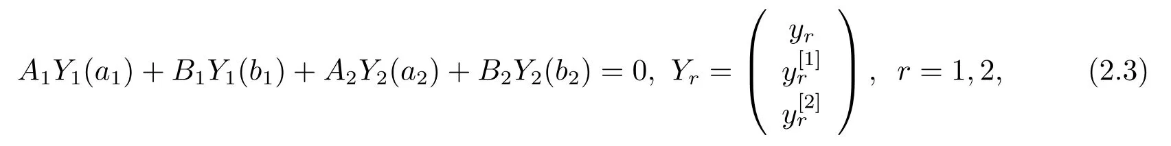
Consider the boundary value problem (BVP)
where

with the boundary conditions
hereare quasi-derivatives.
Generally speaking, if the matricesA1, B1, A2, B2∈M6×3(C) in the boundary conditions (2.3) satisfy the conditions
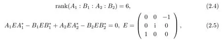
then boundary conditions(2.3)are called self-adjoint boundary conditions,where“?”denotes conjugate transpose of the value.
In the present paper, we will consider the self-adjoint boundary conditions (2.3)-(2.5)under the following two cases:
Case 1 The separated boundary conditions:
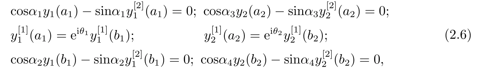
where 0≤α1,α3<π,0<α2,α4≤π,0<θ1,θ2<π.
Case 2 The coupled boundary conditions:
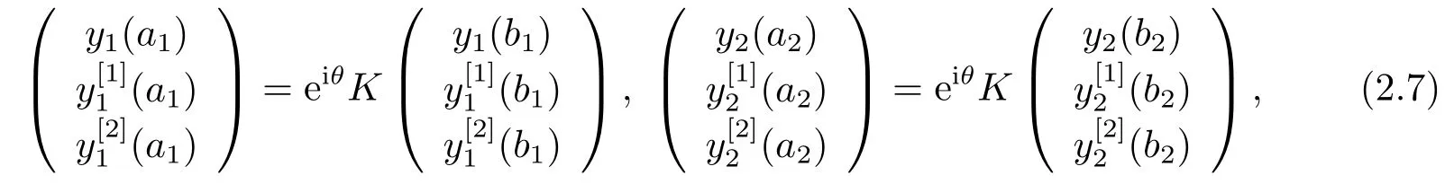
wherekij ∈R,det(K)=1,and?π<θ <0 or 0<θ <π.
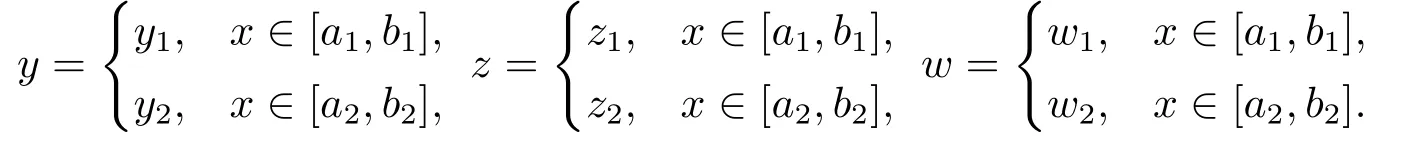
Let the weighted space be defined as
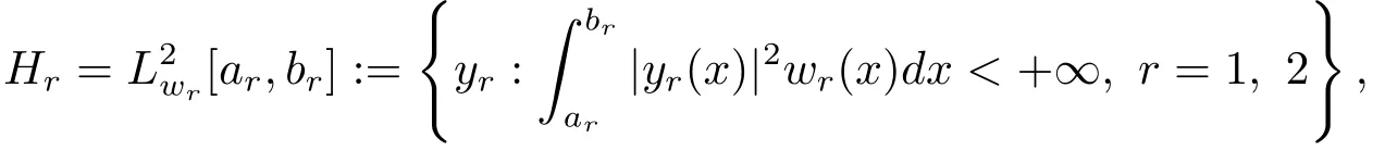
and define

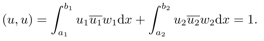
with the inner product
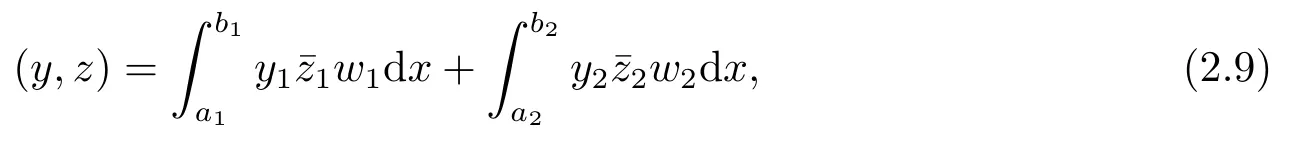
where
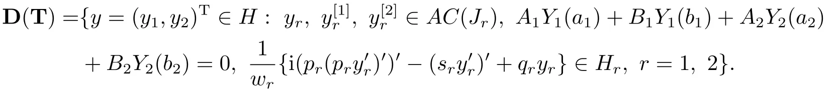
For anyy=(y1, y2)T∈H,define an operator T as

with the domain
3.The Continuity of Eigenvalues and Eigenfunctions
In this section we consider the continuous dependence of the eigenvalues on the parameters of BVP (2.1)-(2.3).
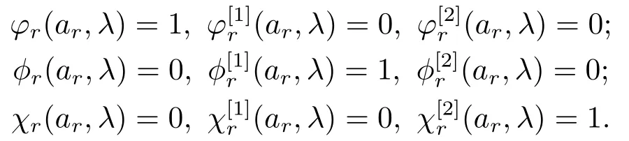
Letφr,φr,χr(r= 1,2) be the fundamental solutions of the equation (2.1) on [ar,br]satisfying the initial conditions
Definer=1,2,thenΦ(x,λ) is the fundamental solution matrix of equation (2.1) satisfying initial conditionsΦ(ar,λ)=IonJ, whereIis the identity matrix.
Lemma 3.1The complex numberλis an eigenvalue of BVP (2.1)-(2.3) if and only if the equality

holds.
ProofLet
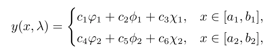
wherec1,c2,c3,c4,c5,c6∈C.Thenλis an eigenvalue of BVP (2.1)-(2.3) if and only if there exists non zero constant vector (c1,c2,c3,c4,c5,c6)T0 such thatysatisfies (2.1)-(2.3).It follows from the boundary conditions (2.3) that
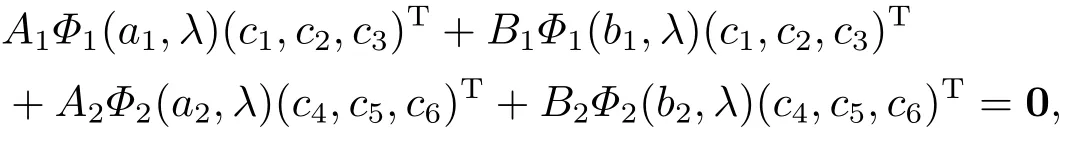
then

Because (c1,c2,c3,c4,c5,c6)T0, Δ(λ)=0.This completes the proof.
Consider a Banach space
X=R4×M6×3(C)×M6×3(C)×M6×3(C)×M6×3(C)×L(J)×L(J)×L(J)×L(J)
with the norm

w=
For anyω=(a1,b1,a2,b2,A1,B1,A2,B2,,s,q,w)∈X, let

Theorem 3.1Letω0= (a10,b10,a20,b20,A10,B10,A20,B20,s0,q0,w0)∈Ω,and suppose thatμ=λ(ω)is the eigenvalue of BVP(2.1)-(2.3).Thenλis continuous atω0.That is, given anyε>0,there exists aδ >0 such that ifω ∈Ωsatisfies
‖ω ?ω0‖<δ,
then
|λ(ω)?λ(ω0)|<ε.
ProofFrom Lemma 3.1,μis an eigenvalue of BVP(2.1)-(2.3)if and only if Δ(ω0,μ)=0.According to the theory of one interval, we know that for anyω ∈Ω, Φ1(b1,λ(ω)) andΦ2(b2,λ(ω)) are all entire functions ofλand are continuous atω ∈Ω.So Δ(ω,λ(ω)) is also an entire function ofλand it is continuous inω.It is obvious that Δ(ω0,λ) is not constant.Hence there existsρ >0 such that Δ(ω0,λ)forλ ∈Sρ:={λ ∈C:|λ ?μ|=ρ}.By the well known theorem on continuity of the roots of an equation as a function of parameters,the statement follows.
Lemma 3.2Letω0= (a10,b10,a20,b20,A10,B10,A20,B20,s0,q0,w0).Letλ=λ(ω)be an eigenvalue of BVP (2.1)-(2.3).Ifλ(ω0) is simple, then there exists a neighborhoodMofω0inΩsuch thatλ(ω) is simple for everyωinM.
ProofThe proof can be given similarly as in [9], only to note the case should be extended from one interval case to two-interval case.
By a normalized eigenfunctionuof BVP (2.1)-(2.3) we mean an eigenfunctionuthat satisfies
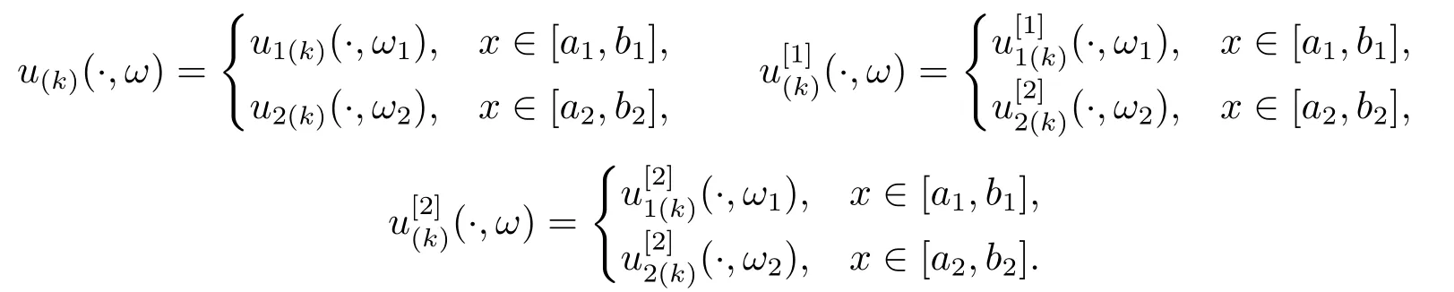
Theorem 3.2Let the hypotheses and notation of Theorem 3.1 hold,and the multiplicity ofλ(ω) is the highest multiplicity ofλ(ω1) andλ(ω2).LetM ?Ωbe a neighborhood ofω0,and if the multiplicity of eigenvalueλ(ω) isl(l= 1,2,3) for anyω ∈M, then there arellinearly independent normalized eigenfunctionsu(k)=u(k)(·,ω), k= 1,··· ,l,ofλ(ω), whenω →ω0, it has

all uniformly on any compact subintervals ofJ, where
In particular, ifλ(ω0) is a simple eigenvalue, then forω ∈M ?Ω,λ(ω) is also simple.There is a normalized eigenfunctionu(1)(·,ω) such that whenk=1, (3.1) hold.
Proof1) Supposeλ(ω0) is simple, then by Lemma 3.2, there exists a neighborhoodMofω0such thatλ(ω) is simple for allω ∈M.For allω ∈M, choose an eigenfunctionu=u(·,ω) ofλ(ω) satisfying

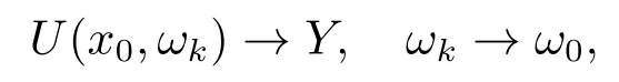
wherex0is any point inJ,U(x,ω)=
It suffices to show that

If (3.2) does not hold, then there exists a sequence{ωk}?Ωsuch that
wherer= 1,2.YandU(x0,ω0) are linearly independent vectors in C3due to the normalization atx0.
LetZbe the vector solutions of (2.1) with the sameω=ω0, λ(ω0) determined by the initial conditionZ(x0)=Y, wherer=1,2.
According to the continuity theorem of solutions to initial values and parameters,U(x,ωk)→Z(x) uniformly on any compact subinterval ofJask →∞, namely that
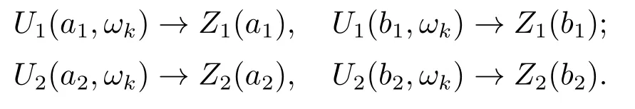
BecauseU(·,ωk) satisfies the boundary conditions,

Letk →∞,then

Therefore,Zis a vector eigenfunction forω=ω0andλ=λ(ω0), which is linearly independent ofU(·,ω0).This contradicts the fact thatλ=λ(ω0) is simple.
2) Suppose the multiplicity of eigenvalueλ(ω) islfor allω ∈M.Then we can choose eigenfunctionsu(·,ω) ofλ(ω), all of which satisfy the same initial condition atc0for somec0∈Jsince a linear combination ofllinearly independent eigenfunctions can be chosen to satisfy arbitrary initial conditions.Similar to the above discussion, the corresponding conclusion can be obtained.
4.Differential Expression of Eigenvalues
Definition 4.1A mapTfrom a Banach spaceXinto another Banach spaceYis differentiable at a pointx ∈Xif there exists a bounded linear operatordTx:X →Y,such that forh ∈X

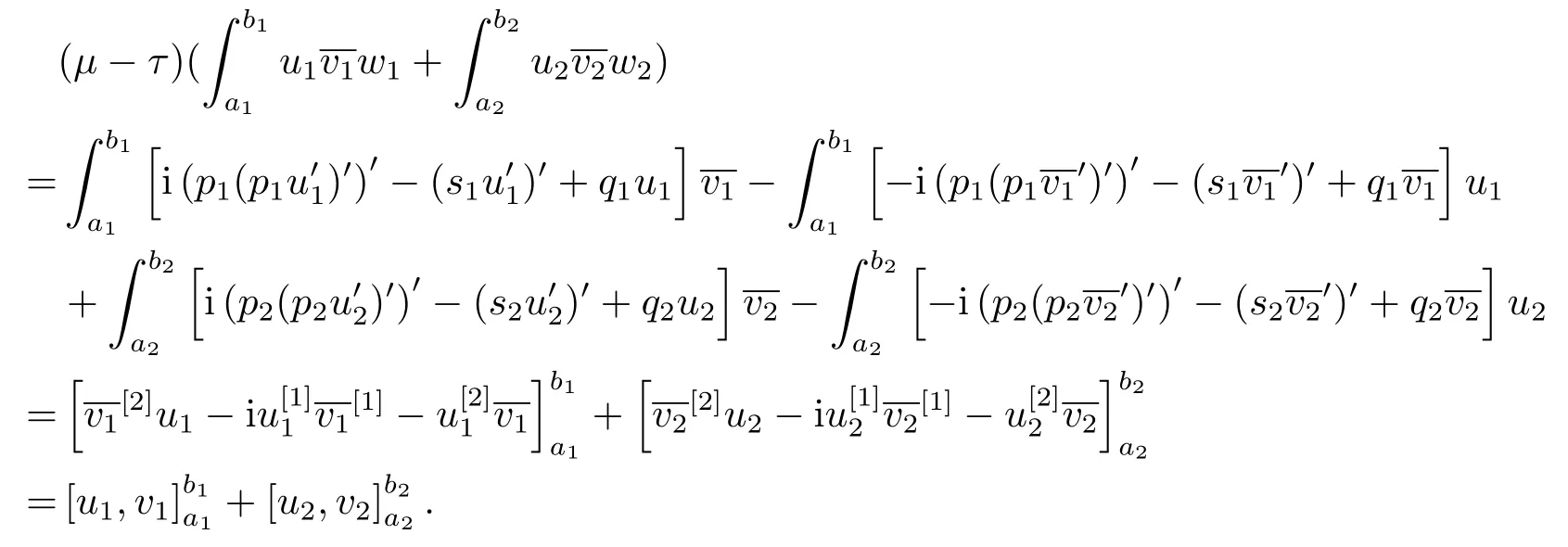
Lemma 4.1Letλ=μandλ=τbe the eigenvalues of BVP (2.1)-(2.3),uandvare the eigenfunctions corresponding toμandτ, respectively, then
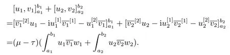
ProofAccording to the method of integration by parts
Theorem 4.1Letλ(ω)be an eigenvalue of BVP(2.1)-(2.3)withω ∈Ω,andu=u(·,ω)be a normalized eigenfunction forλ(ω).Thenλis differentiable with respect to all parameters inω, and more precisely, the derivative formulas ofλare given as follows:
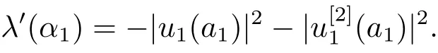
1) Fix all parameters ofωexceptα1and letλ=λ(α1) be the eigenvalue of BVP (2.1)-(2.3), andu=u(·,α1) the normalized eigenfunction.Then

2) Fix all parameters ofωexceptα2and letλ=λ(α2) be the eigenvalue of BVP (2.1)-(2.3), andu=u(·,α2) the normalized eigenfunction.Then

3) Fix all parameters ofωexceptα3and letλ=λ(α3) be the eigenvalue of BVP (2.1)-(2.3), andu=u(·,α3) the normalized eigenfunction.Then

4) Fix all parameters ofωexceptα4and letλ=λ(α4) be the eigenvalue of BVP (2.1)-(2.3), andu=u(·,α4) the normalized eigenfunction.Then

5) Fix all parameters ofωexceptθ1and letλ=λ(θ1) be the eigenvalue of BVP (2.1)-(2.3), andu=u(·,θ1) the normalized eigenfunction.Then

6) Fix all parameters ofωexceptθ2and letλ=λ(θ2) be the eigenvalue of BVP (2.1)-(2.3), andu=u(·,θ2) the normalized eigenfunction.Then

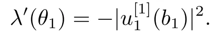
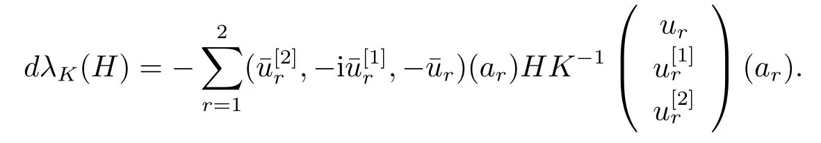
7) Fix all parameters ofωexceptKand letλ=λ(K) be the eigenvalue of BVP (2.1)-(2.3), andu=u(·,K) the normalized eigenfunction.Then
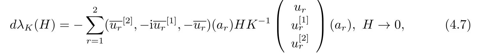
where det(k)=det(k+H)=1;
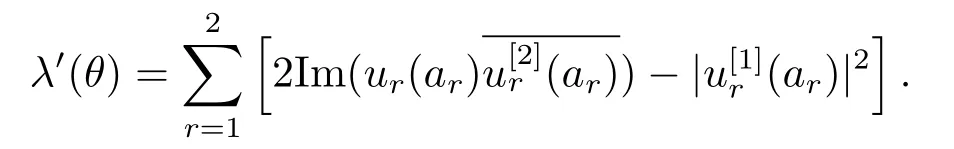
8)Fix all parameters ofωexceptθand letλ=λ(θ)be the eigenvalue of BVP(2.1)-(2.3),andu=u(·,θ) the normalized eigenfunction.Then

9) Fix all parameters ofωexcepts1and letλ=λ(s1) be the eigenvalue of BVP (2.1)-(2.3), andu=u(·,s1) the normalized eigenfunction.Then

10) Fix all parameters ofωexcepts2and letλ=λ(s2) be the eigenvalue of BVP (2.1)-(2.3), andu=u(·,s2) the normalized eigenfunction.Then

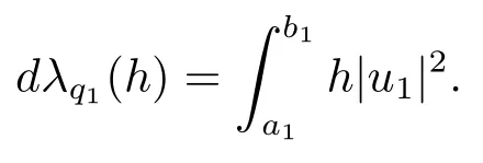
11) Fix all parameters ofωexceptq1and letλ=λ(q1) be the eigenvalue of BVP (2.1)-(2.3), andu=u(·,q1) the normalized eigenfunction.Then

12) Fix all parameters ofωexceptq2and letλ=λ(q2) be the eigenvalue of BVP (2.1)-(2.3), andu=u(·,q2) the normalized eigenfunction.Then

13) Fix all parameters ofωexceptw1and letλ=λ(w1) be the eigenvalue of BVP(2.1)-(2.3), andu=u(·,w1) the normalized eigenfunction.Then

14) Fix all parameters ofωexceptw2and letλ=λ(w2) be the eigenvalue of BVP(2.1)-(2.3), andu=u(·,w2) the normalized eigenfunction.Then

ProofSince the proof of (4.1)-(4.4) are the same, here we just prove (4.1).
For anyε ∈R sufficiently small, letu=u(·,α1) andv=u(·,α1+ε) denote the normalized eigenfunctions ofλ(α1) andλ(α1+ε),respectively, then
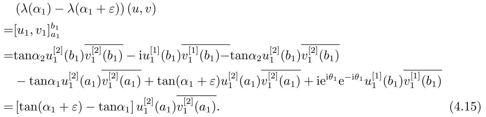
Dividing both sides of (4.15) byεand taking the limit asε →0, by Theorem 3.2 we get
To prove (4.5), for anyh ∈R sufficiently small, letu=u(·,θ1) andv=u(·,θ1+h)denote the normalized eigenfunctions ofλ(θ1) andλ(θ1+h), respectively, then
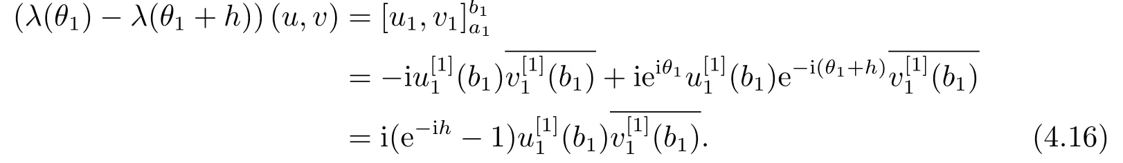
Dividing both sides of (4.16) byhand taking the limit ash →0, by Theorem 3.2 we get
The proof of (4.6) is similar to that of (4.5) and hence omitted.
To prove (4.7), letu=u(·,K),v=u(·,K+H) denote the normalized eigenfunctions ofλ(K) andλ(K+H), respectively.
From the boundary condition, we have
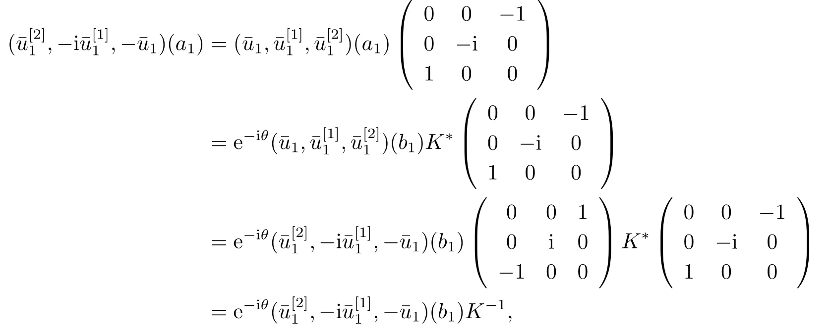
i.e.,

Since
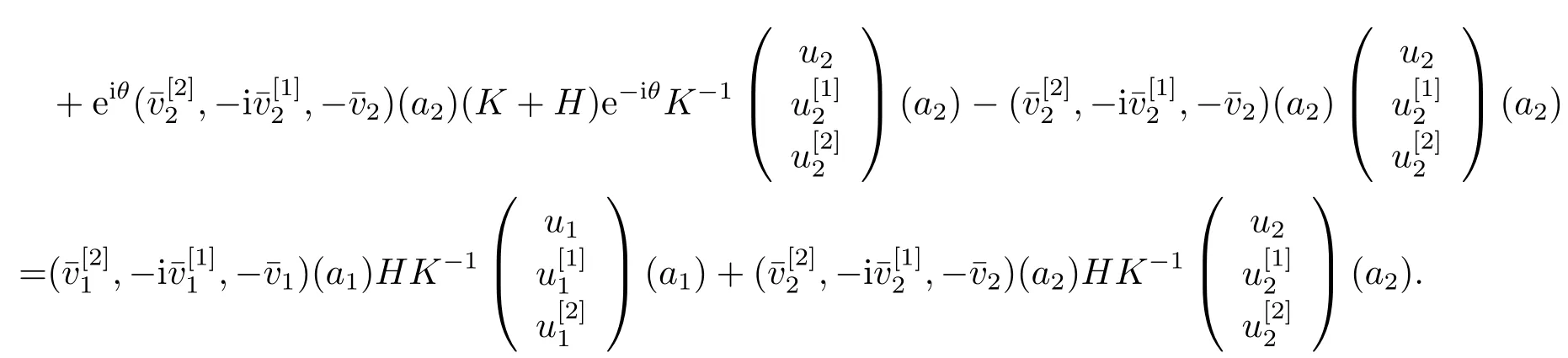
Then letH →0, we can get
To prove (4.8), for anyh ∈R sufficiently small, letu=u(·,θ),v=u(·,θ+h) denote the normalized eigenfunctions ofλ(θ) andλ(θ+h), respectively, then

Dividing both sides of (4.17) byhand taking the limit ash →0, we get
Since the proof of (4.9)-(4.14) is the same, here we only prove (4.11).
For anyh ∈L(J), letu=u(·,q1),v=u(·,q1h) denote the normalized eigenfunctions ofλ(q1) andλ(q1h), respectively, whereq1h=q1+h, then
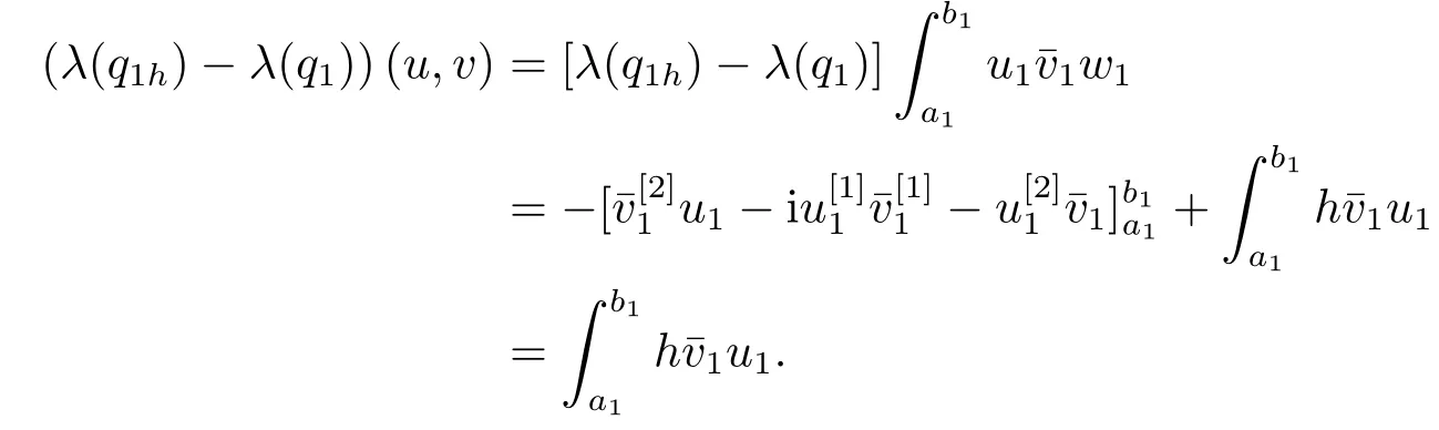
Ash →0, we obtain
- 應(yīng)用數(shù)學(xué)的其它文章
- 基于不確定控制理論的最優(yōu)策略研究
- 一類擬線性薛定諤方程非平凡解的存在性
- The Optimal Error Estimates for the Dynamic Magnetic Field of Solar Interface Problem by H(curl,Ω) Finite Element Methods
- 協(xié)變量維數(shù)可以趨于無窮的縱向數(shù)據(jù)的廣義估計方程分析
- 不可壓磁流體力學(xué)方程組的高精度數(shù)值解法
- Error Analysis of Kernel Regularized Regression with Deterministic Spherical Scattered Data