YAO Changhui(姚昌輝) SHEN Junwen(申俊文) ZHAO Yanmin(趙艷敏)

(1.School of Statistics and Big Data, Zhengzhou College of Finance and Economics,Zhengzhou 450000, China; 2.School of Mathematics and Statistics, Zhengzhou University,Zhengzhou 450001, China; 3.School of Science, Xuchang University, Xuchang 461000, China)

Abstract: In this paper, the interface edge element is utilized to approach the dynamic magnetic field of solar interface problem, which has optimal interpolation approximation.And, the domain is partitioned by interface-aligned triangulation with jump interface surrounded by δ-strip.Based on properties of interface edge element, the optimal error estimates of the dynamic magnetic field is obtained with convergent rate O(τ +h), where τ,h are subdivision step in time and space, respectively.At last, numerical simulations of the dynamic magnetic field of solar interface model is shown.

Key words: Interface edge element; Solar interface problem; Optimal error estimate;Dynamic magnetic field

1.Introduction

The intense magnetic activities in the deep interiors of sun can be formulated by the model of the dynamic magnetic field of solar interface[1?2], which is generally called Jupiter’s magnetic field[3].Such a nonlinear model describes the convective instability concluding a small-scale turbulent flows and large-scale global circulations.Therefore, this kinematic dynamo consists of three major zones in spherical geometry: The inner radiative sphere with the interior magnetic diffusivity,the annular region with the turbulent convection zone and the global circulation,and the outer exterior region with the another different magnetic diffusivity.Mathematically, this is a nonlinear interface problem with discontinuous coefficients.

The Maxwell’s equations with discontinuous coefficients was approximated in[4]by edge element method classically.This solar dynamic interface problem was firstly analyzed and simulated by Lagrange mixed finite element methods numerically in [2, 5], where a convergent rateO(τ+0≤s <1 was obtained arduously.The crucial reason is that the given interface element has not an optimal interpolation property as the classical.Precisely speaking, they employed the popular Hood-Taylor in [6] and used modifying the Scott-Zhang interpolation operator in [7] on the interface element.Sequently, a new lowest order Ndlec confirming finite element was constructed to approach H(curl,Ω) elliptic interface problem with smooth interfaces in general three-dimensional polyhedral domains.The interpolation approximate of this new interface edge element isO(h) by theδ-strip technique.It is obviously that the convergent rate in [5] is not optimal.Other interface elements can be found,for example, Poisson problems[8?10], fluid flows problem[11?12], Maxwell’s equation[13?14].

In this paper, we employ the interface edge element byδ?strip strategy to reanalyze the model of the dynamic magnetic field of solar interface.The domain is partitioned by interfacealigned triangulation.By a novel interpolation approximation, we can get an optimal error estimates in temporal and spatial.Compared with the method in [5], the new technique of nonlinear error estimates is direct.Finally, a simple numerical experiment to simulate the dynamic magnetic field of solar interface model.

2.Model, Interface Edge Element and Lemmas

The governing equation of the dynamic magnetic field of solar interface problem can be formulated by

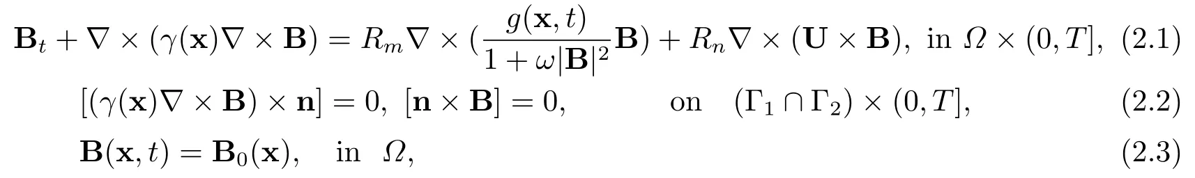
where the domain isΩ=Ω1∪Ω2∪Ω3, Γ1denotes the interface between the inner core and outer convection zone, Γ2stands for the interface between the convection zone and the outer exterior.B is the large-scale magnetic field satisfying?·B=0.γ(x) is the magnetic diffusivity which jumps across the interfaces Γ1and Γ2.The parametersRmandRnare the dynamo parameter in connection with the generation process of small-scale turbulence and is the magnetic Reynolds number associated with the global circulation, respectively.g(x,t)is a model-oriented function, andω >0 is a constant.The nonlinear termis derived from the alpha quenching[1], the termdescribes the turbulent convection flow as well asRn?×(U×B) standards for the global circulation.[w] represents the quantity of jumps of w across the interfaces and n means the unit outward normal.

For convenience of expression, we define some notations, which are adopted in [15].

Then the variational formula of the equations (2.1)-(2.2) can be written by:?t ∈(0,T],find B∈V such that

For the different regionΩ1,Ω2,Ω3, we employδ-strip regions around the interface (Fig.2.1(b)).For the mesh partition of the domain, we also adopt the concept ofinterface-alignedtriangulation(Fig.2.1(c)),the assumptions and definitions in[15]in order to avoid repetition.If we employ the lowest first type Nedelec’s element space Vh, which preserves the curl-free property of a grad field to deal with the property?·B = 0, interface-aware interpolation operators can be given by: VVhlike [15].This operator has an interpolation error constrained byδas follows.

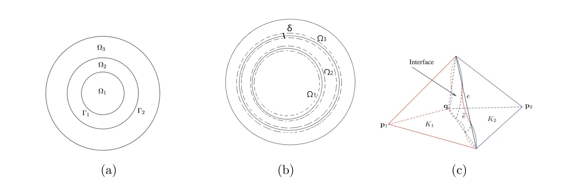
Fig.2.1 (a) Domain Ω = Ω1∪Ω2∪Ω3: inner region Ω1, convective region Ω2, outer region Ω3; (b) δ-strip regions around the interface; (c) Two twin interface elements K1 and K2

Lemma 2.1Under the assumption w∈V,there exists a positive constantCsuch that

whereδ >0 is the thickness ofδ-strip regions.

For the convenience of next section, we need the following lemma in [16].

Lemma 2.2For the vector A, B and the parameterγ >0, there holds

3.Error Estimates

To formulate a fully discrete scheme, we divide the time interval [0,T] into uniform subintervals by points 0 =t0< t1< ··· < tN=T,wheretn=nτ, n= 0,··· ,N,andτ=T/Ndenotes the time step size.We also define the following notations

The back-Euler finite element scheme of the equations(2.1)-(2.2)can be formulated: For, find∈Vhsuch that

Now we present the optimal convergent result.

Theorem 3.1Let Bn ∈L∞(0,T;(H1(curl;Ωk))),k= 1,2,3,be the solution of the equation (2.4) at timet=tn,n= 0,1,2,··· ,N.Letbe the finite element solution of the discrete scheme (3.1).Under the assumptions Bt ∈L∞(0,T;H1(curl;Ωk)),Btt ∈L∞(0,T;L2(Ωk)),k=1,2,3, there holds the optimal error estimate

whereCis a positive constant independent of mesh sizehand the time stepτ.

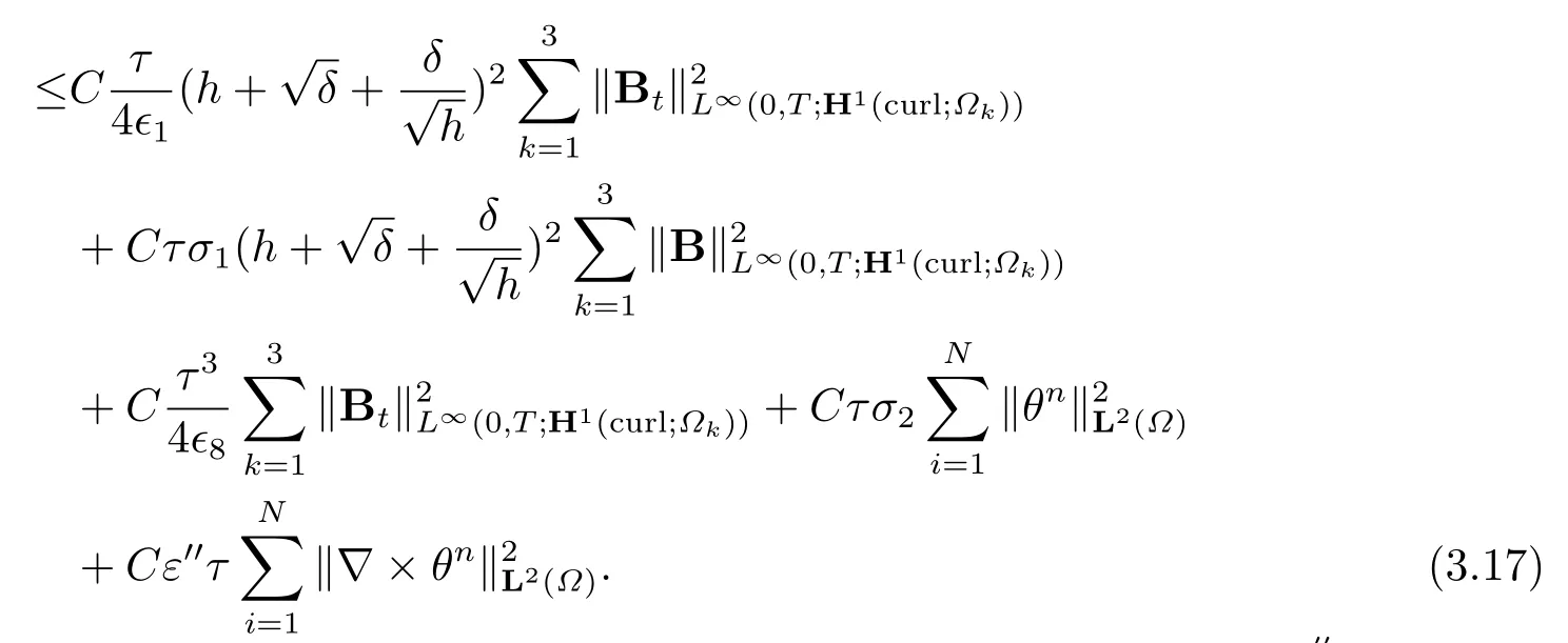
By Lemma 2.1, Lemma 2.2 and Young’s inequality,we have the following error estimates

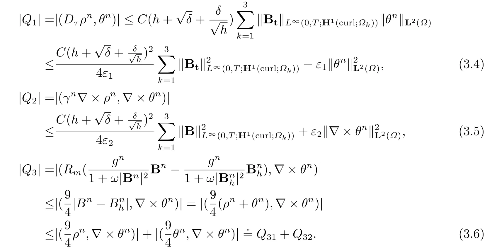
Two terms in (3.6) can be estimated by

respectively.

Summing (3.7) and (3.8) yields

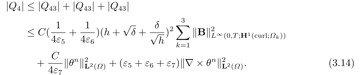
For the estimates ofQ4in (3.3), there holds

Three terms in (3.10) can be controlled by the following error estimates

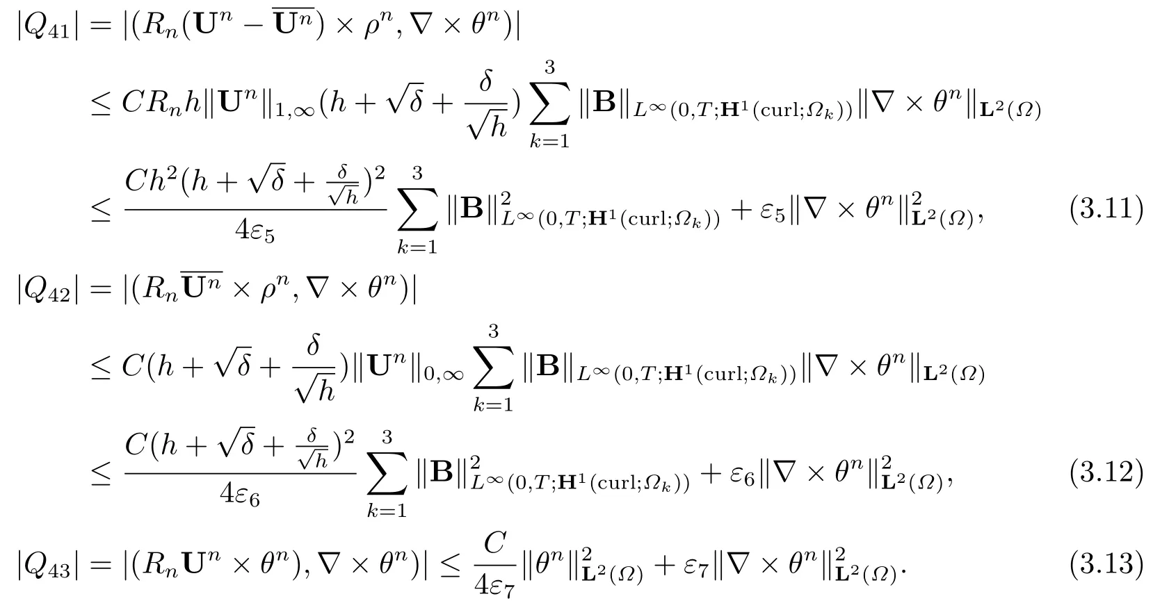
The estimates results (3.11)-(3.13) can lead to

The termQ5in (3.3) can be estimated directly by the Taylor formula

The left terms in (3.3) can be estimated by

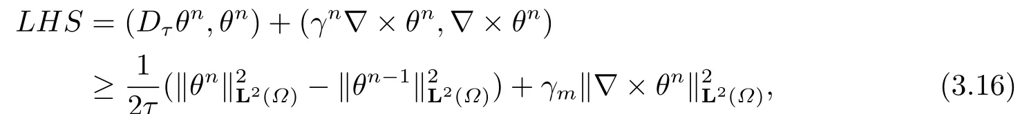
where the parameterγsatisfyingγm ≤γ ≤γM, andγm,γMare positive constants, respectively.

Denoting

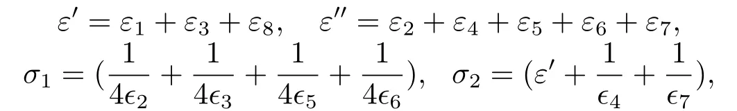
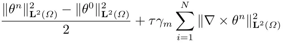
multiplyingτin (3.4),(3.5),(3.9),(3.14) (3.15) and (3.16), and summing up from 1 tom,n ≤m ≤N, we obtain that

Fromθ0= 0, taking the small time sizeτand the proper parameterssuch thatγm ?Cτ?′′ >0 and Grall’s inequality, we conclude the proof.

Theorem 3.2Under the assumption of Theorem 3.1, if the thickness parameter is taken byδ=O(h2), then there holds

whereCis a positive constant independent of mesh sizehand the time stepτ.

ProofTaking the thickness parameter is taken byδ=O(h2), from Lemma 1 and triangle inequality, we can complete the proof.

RemarkFrom Theorem 3.1 and Theorem 3.2,we can obtain the optimal error estimates by the lowest interface edge element.Obviously, the convergent rate isO(τ+h), which is higher thanO(τ0≤s <1 in [5].Employing the Crank-Nicolson discrete scheme in time[16?18], the convergent rate will beO(τ2+h).The corresponding proof is left to the readers.

4.Numerical Experiments

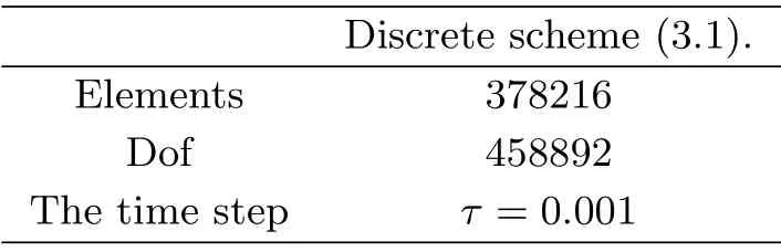
Tab.4.1 Comparison of computational costs

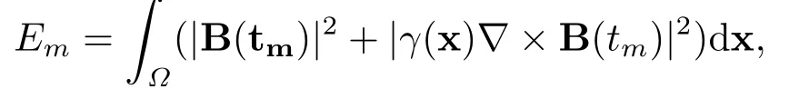
If the magnetic energy is defined by the evolution of the magnetic energyEmof the dynamo for different values ofRmis displayed in Fig.4.1.The computational results for the related component of the solutions is displayed in Fig.4.2.

Fig.4.1 (a) Domain Ω =Ω1 ∪Ω2 ∪Ω3; (b) The evolution of the magnetic energy Em of the dynamo for different values of Rm

Fig.4.2 Contours of the |B| in z =0 for t=0.2:0.2:2.4 ( from (a) to (l)) for Rm=100