Regularization Method and A-posteriori Convergence Estimate for a Space-fractional Diffusion Problem Backward in Time
2022-01-19 06:23:44ZHANGHongwu張宏武LVYong呂擁
應(yīng)用數(shù)學(xué) 2022年1期
ZHANG Hongwu(張宏武), LV Yong(呂擁)
(School of Mathematics and Information Science, North Minzu University,Yinchuan 750021, China)
Abstract: The article researches a space-fractional diffusion problem backward in time.Based on the result of conditional stability,we develop a generalized Tikhonov regularization method to overcome the ill-posedness of this problem, and then obtain the convergence estimates of logarithmic and double logarithmic types for the regularized method by the a-posteriori choice rules of regularization parameter.Some results of numerical simulations verify the convergence and stability for this method.
Key words: Ill-posed problem; Space-fractional diffusion problem; Regularization method; A-posteriori convergence estimate; Numerical simulation
1.Introduction
The space-fractional diffusion equation is generally used to describe some diffusion phenomena, such as the super-diffusion, non-Gaussian diffusion, sub-diffusion, etc.In the past years, the direct problems for this equation have been studied extensively.In recent years,more and more people are focusing on the inverse problems for this equation, which usually include parameter identification problem, inverse initial value problem, Cauchy problem, inverse heat conduction problem, inverse source problem, inverse boundary condition problem,and so on.
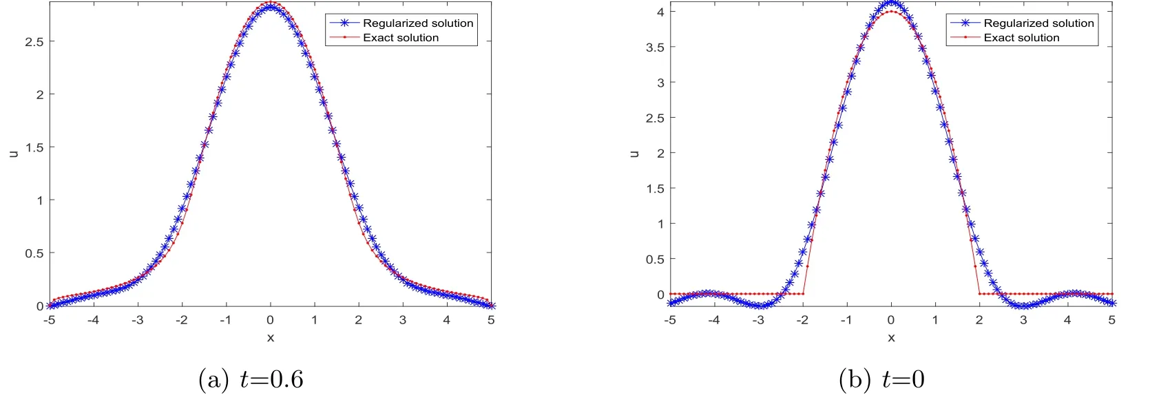
This article considers the following space-fractional diffusion problem backward in time
whereT >0 is a constant, 1/2< α ≤1, the one-dimensional fractional Laplacian is defined pointwise by the principal value integral[1]

According to the Fourier transform,it easily can be known that the fractional Laplacian is the symmetric case (θ=0) of the Riesz-Feller fractional derivativexDαθdefined in [2].This kind of fractional derivative has wide applications in some important science fields, such as the theory of probability distribution, ecology, plasma physics, continuum mechanics, hydrology,and so on.
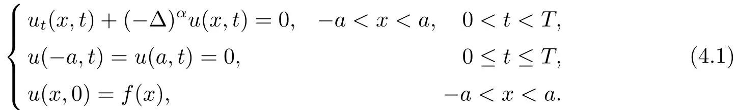
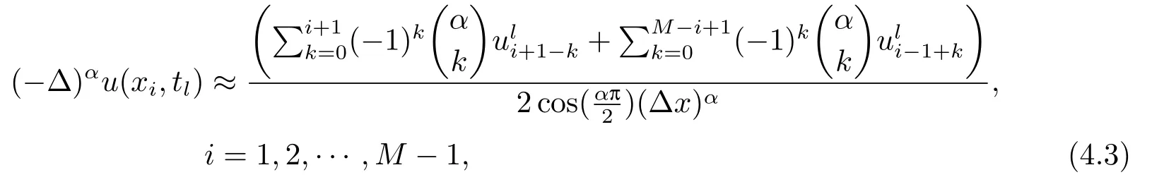
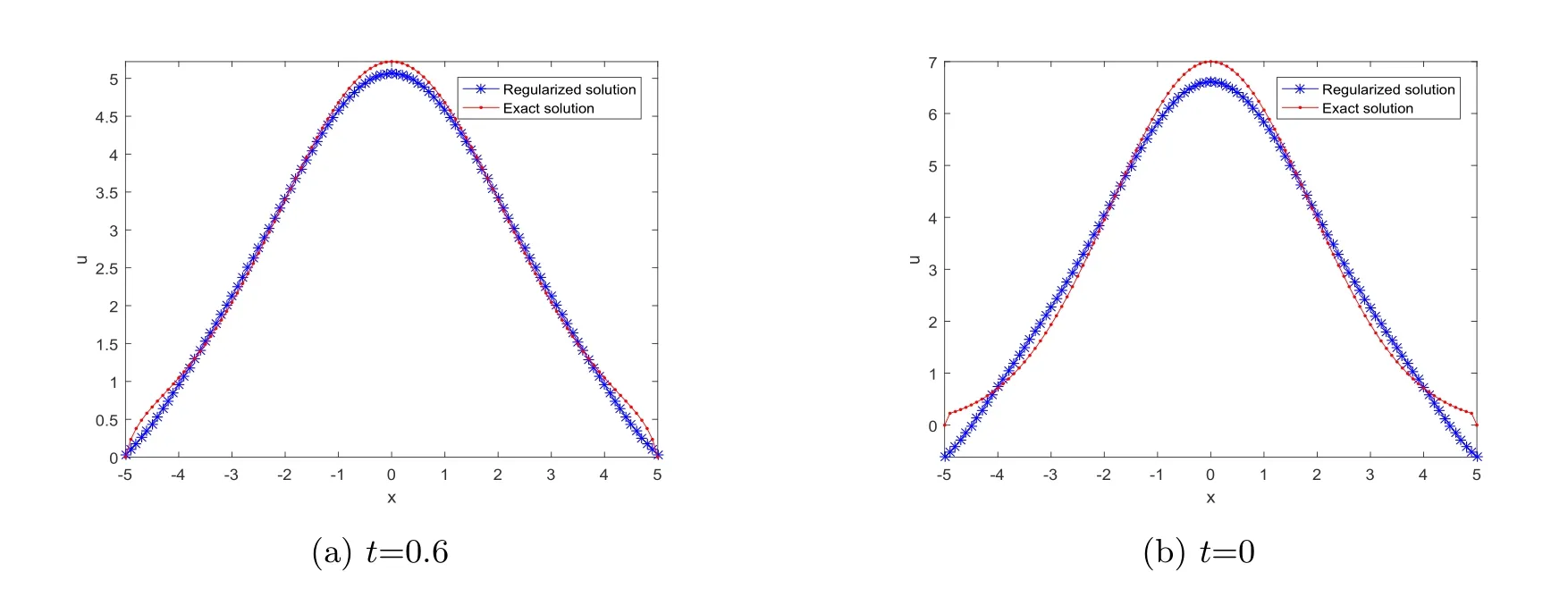
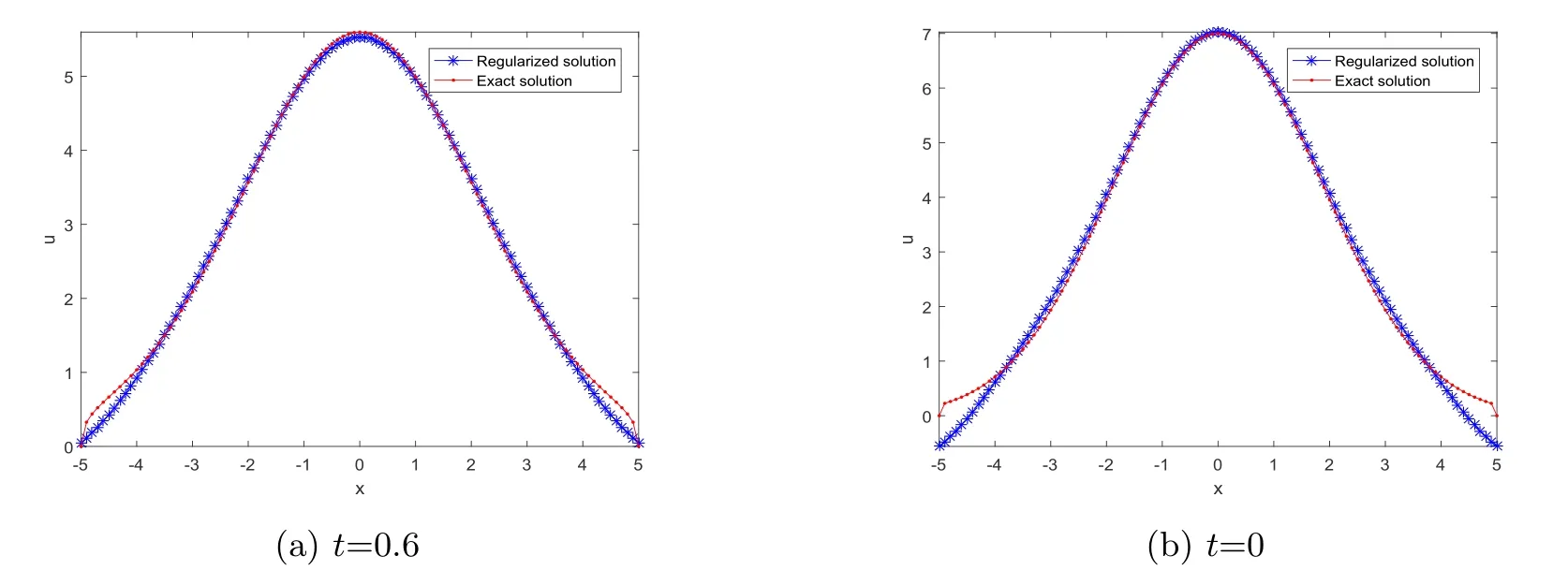
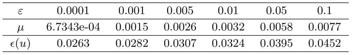
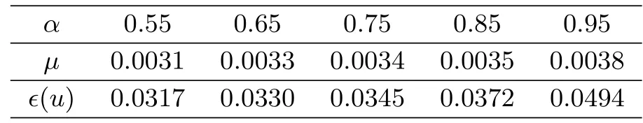
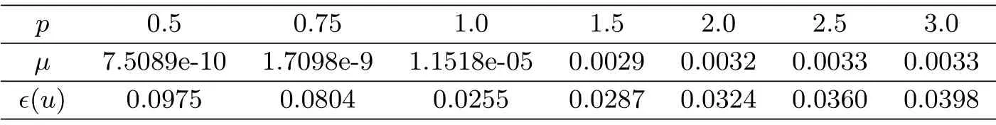
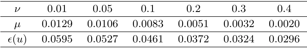
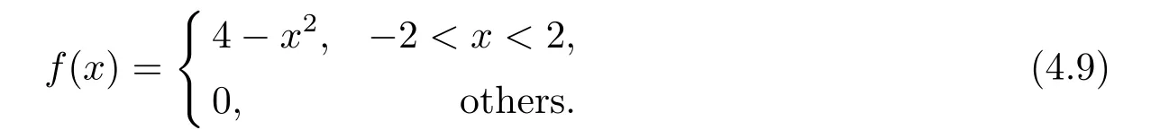
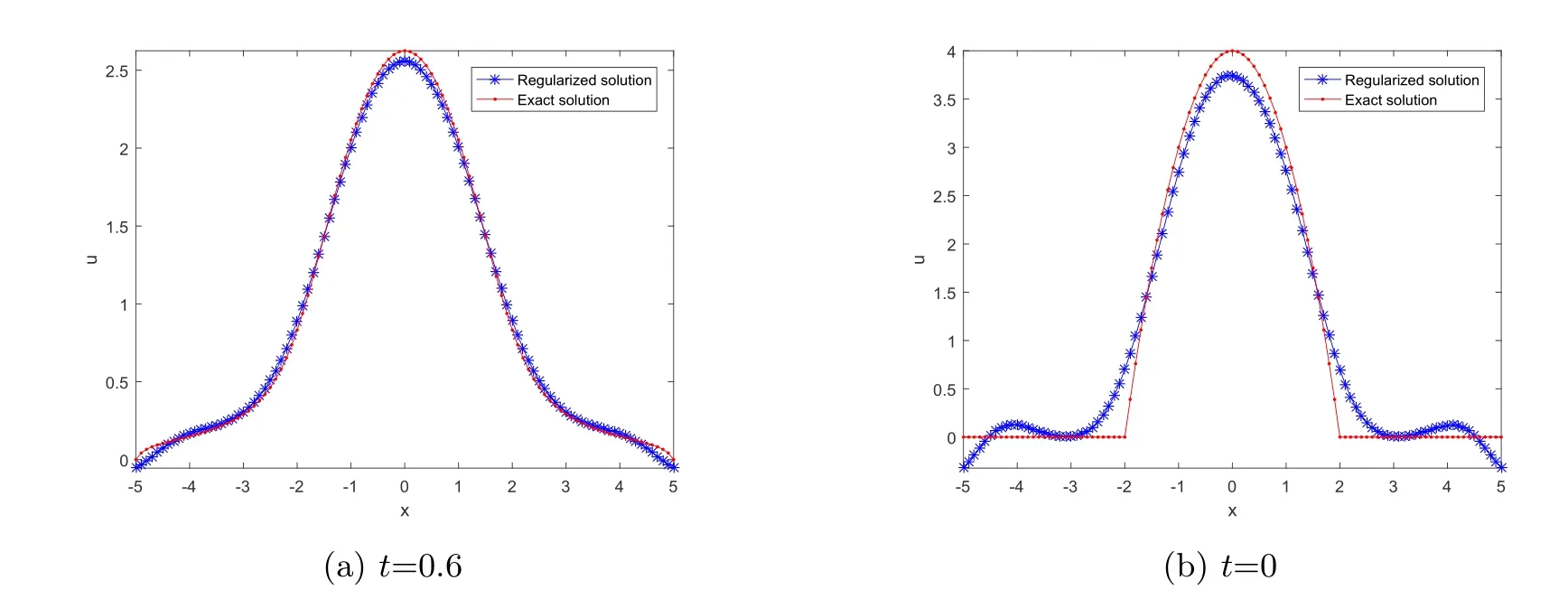
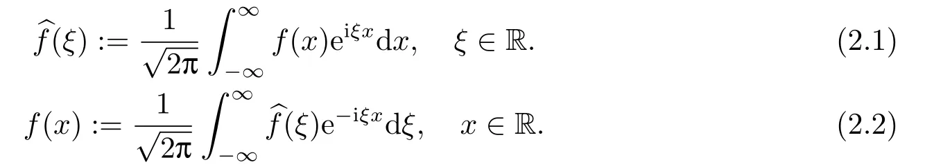
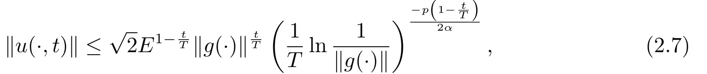
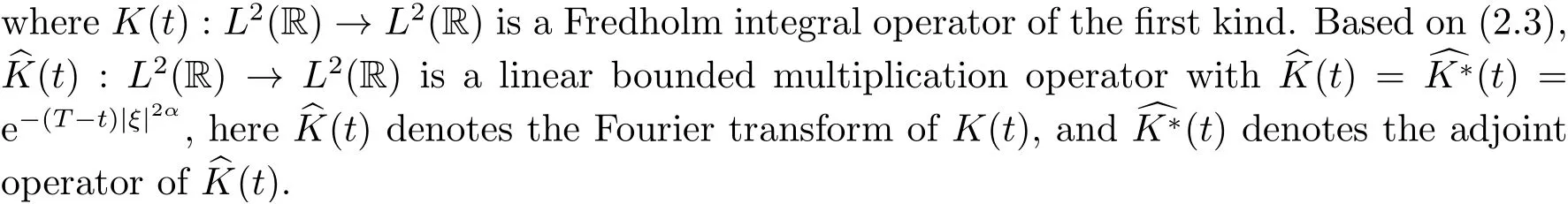
Letδ >0 be the measured error bound, given the final measured datagδ(x) with‖gδ(x)?g(x)‖L2(R)≤δ, our purpose is to determineu(x,t)(0≤t In ordinary Tikhonov regularization method, the penalty term commonly is added asInstead of the Tikhonov method,this paper adds the penalty term as(p>0)to construct a generalized Tikhonov regularization method(Section 2),and derive the convergence estimates of logarithmic and double logarithmic types by adopting an a-posteriori selection rule of regularization parameter.Finally, we verify the computational effectiveness for our method by making the corresponding numerical experiments. Ⅰ Conditional stability Letf ∈L2(R), the Fourier transform and inverse Fourier transform are defined as Take the Fourier transform of problem(1.1)with respect tox,then forξ ∈R,the solution of problem (1.1) in the frequency domain can be expressed as below hence, the exact solution of problem (1.1) can be written by From (2.4) we know that, as|ξ|→+∞, the high frequency part of function e(T ?t)|ξ|2αtends to infinity, hence the problem (1.1) is ill-posed in the sense that the solution does not depend continuously on the given data.However, under certain additional condition, we can obtain the continuous dependence of solution, which is called as the conditional stability. Suppose that there exists a constantE >0, such that the following a-priori bound holds here‖u(·,0)‖pdenotes the Sobolev spaceHp-norm defined by In [12], under the assumption of the a-priori bound condition (2.5), the authors established the condition stability for problem (1.1) by using the interpolation method. Theorem 2.1[12]Assume the a-priori bound condition (2.5) be valid, then the below result of condition stability holds where,‖·‖denotes theL2-norm. Ⅱ Regularization method According to the expression of solution (2.4), in order to overcome the ill-posedness of the considered problem, a natural way is to eliminate the high frequency part (|ξ|→+∞) of function e(T ?t)|ξ|2αand construct a stable approximation solution of problem (1.1). Below,based on the condition stability(2.7),we make a description for our regularization method.According to (2.4), for the fixed 0≤t Assume the noisy datagδsatisfies In order to get a stable solution to the problem (1.1), we solve the variational problem whereμ >0 plays a role of the regularization parameter,δ >0 denotes the measured error bound.By the Parseval identity and (2.3), this variational problem becomes minimizing the functional From (2.12), in the frequency domain the regularized solutionξ,t) can be expressed as thus, the regularization solution of problem (1.1) can be written as Remark 2.1Note that, in (2.10), we add the penalty item in the sense ofHp-norm to construct the regularization solution (2.14).In fact, if we add the penalty item in the sense ofL2-norm, i.e., the standard Tikhonov regularization method as follow the regularization solution can be expressed as If settingt= 0 and making a modification on (2.16), we can obtain the simplified Tikhonov regularized solution From (2.14), (2.16) and (2.17), we can find that, in order to overcome the ill-posedness of the considered problem(i.e.,eliminate the high frequency part of function e(T ?t)|ξ|2α),the functionis a better “kerne” thanandand asp= 0, our method just is the simplified Tikhonov method, thus the method given in this paper is an interesting and meaningful one,which is similar with the generalized Tikhonov method in[13].In 2012, [14]used a similar method to research a multidimensional inverse source problem for standard heat equation (the main equation isut(x,t)?Δnu(x,t)=f(x),x∈Rn,0 Remark 2.2In addition, we point that our method also can be extend to multidimensional case.For instance, the two-dimensions problem inL2(R2):ut=?r(?Δ)βu,t >0,u(x,y,T) =g(x,y), where 0< β ≤1,r >0 is a constant, and the fractional differential operator(?Δ)βis defined as(?Δ)βu(x,y)=∫R2(4π2ξ2+4π2η2)β^u(ξ,η)e2πi(ξx+ηy)dξdη.However, because the special process is similar to one-dimensional case, this paper only considers the problem (1.1). This section adopts a kind of a-posteriori rule to select the regularization parameterμ, this idea comes from [4], and then derives the convergence estimate for the regularization method.On the general description for the a-posteriori selection rule of regularized parameter,we can see the discrepancy principle in [15].We select the regularized parameterμby the following equation here,h(δ)>δwill be given later.The following two Lemmas will be needed in the convergence estimate of a-posteriori type. Lemma 3.1Let?(μ) =(x,T)?gδ(x)‖and 0< h(δ)< ‖gδ‖, then we have the following conclusions: (i) Forμ∈(0,+∞),?(μ) is a continuous function; (ii)limμ→0?(μ)=0;(iii) limμ→+∞?(μ)=‖gδ‖; (iv) Forμ∈(0,+∞),?(μ) is a strictly increasing function. ProofWe easily can prove this Lemma by taking here we skip the special procedure.Lemma 3.1 means that, as 0 Lemma 3.2Assume that the a-priori bound condition (2.5) is valid, then the regularized solution (2.14) combining with a-posteriori selection rule (3.1) determine that the regularization parameterμ=μ(δ,gδ) satisfies ProofFrom (3.1), there holds By the basic simplification and using the mean value inequality, it can be gotten that From (3.3) and (3.4), we can derive the result of Lemma 3.2. Theorem 3.1Suppose thatugiven by (2.4) is the exact solution of problem (1.1),uδμdefined by (2.14) is the regularization solution, let the exact datagand measured datagδsatisfy (2.9), and the a priori bound (2.5) is satisfied. (i) If the regularization parameter is selected by a-posteriori rule (3.1) withh(δ) =then we have the following convergence estimate of logarithmic type (ii) If the regularization parameter is chosen by a-posteriori rule (3.1) withh(δ) =δ+then we have the below convergence estimate of double logarithmic type ProofUsing the Parseval theorem, it is clear that Forμ∈(0,1) and from (2.9), we get that By the simple calculation, we notice that, lim|ξ|→0+e?(T ?t)|ξ|2α+(1+|ξ|2)pe(T+t)|ξ|2α= 2,and lim|ξ|→+∞e?(T ?t)|ξ|2α+(1+|ξ|2)pe(T+t)|ξ|2α= +∞, then there exists a positive numberD, such that By (3.9) and Lemma 3.2, we get Now we give the estimate for the second term of (3.7).It is noticed that In addition, according to the a-priori bound condition (2.5), we have By the condition stability result (2.7), it can be gotten that Now, combining (3.10) with (3.13), we can derive that Finally, we can established the convergence results (3.5) and (3.6), respectively. In this section, some numerical experiments are done to verify the accuracy and effectiveness of our method.Since the analytic solution of problem (1.1) is generally difficult to be expressed explicitly, here we solve the following direct problem to construct the final datag(x) by the finite difference method. We choosea= 5,T= 1, denote Δt=and Δx=be the step sizes for time and space variables, respectively.The grid points in the time interval are labeledtl=lΔt,l= 0,1,2,...,L, the grid points in the space interval arexi=?a+iΔx,i= 0,1,2,...,M,and setting=u(xi,tl). We approximateutat (xi,tl) as below and (?Δ)αuat (xi,tl) is approximated as in [3], combining with the boundary condition and initial condition Thus, the final data is given by The measured data is given by the following random form withδ=ε‖g‖, hereεis the noisy level.The regularization solution is calculated by (2.14).For 0< γ <1, we denoteν=the regularized parameter is chosen by the a-posteriori rule (3.1) withh(δ) =δ+δν.We shall make a comparison for the computational results of regularized and exact solutions. For the fixed 0≤t < T, in order to make the sensitivity analysis for numerical results,we calculate the relativeL2-error defined by In the computational procedure, we always take Δx= 1/100, Δt= 1/10000,M= 100,L=10000 andε=0.01. Example 4.1We choose the initial distributionf(x) = 7e?x2/7, and note that it satisfiesf ∈Hp(R)(p>0). Att=0.6 and 0,p=2,numerical results of exact and regularized solutions forα=0.8,1 are shown in Figs.1-2.The regularized parameterμis selected by (3.1) withν=0.3.From Figs.1-2, we can see that this method is feasible and acceptable.Meanwhile, att= 0.6 we also investigate the influences ofε,α,pandνon numerical result.Forα= 0.6,ν= 0.3,p= 2, the relative errors for variousεare shown in Table 1.Table 1 shows that, the better numerical result the smallerεbecomes,this means the convergence of our method.Forp=2,ν=0.3,ε=0.01, the errors for variousαare presented in Table 2.Table 2 indicates that the numerical procedure is stable to the fractional orderα.Forα= 0.6,ν= 0.3,ε= 0.01, the errors for variouspis given in Table 3.Table 3 shows that, in order to obtain the satisfied result, the best value ofpshould be taken as 1, and it has no need to be taken too large.Forα= 0.6,p= 2,ε= 0.01, the errors for variousνis shown in Table 4.From Table 4 we can note that the result becomes well asνbecomes large. Fig.1 α=0.8, p=2: Exact and regularized solutions, the regularized parameter is selected by (3.1) with ν =0.3 Fig.2 α = 1, p = 2: Exact and regularized solutions, the regularized parameter is selected by (3.1) with ν =0.3 Tab.1 At t=0.6: α=0.6, ν =0.3, p=2, the relative errors in L2 norm for various ε Tab.2 At t=0.6: p=2, ν =0.3, ε=0.01, the relative errors in L2 norm for various α Tab.3 At t=0.6: α=0.6, ν =0.3, ε=0.01, the relative errors in L2 norm for various p Tab.4 At t=0.6: α=0.6, p=2, ε=0.01, the relative errors in L2 norm for various ν Example 4.2We take a continuous initial distribution that satisfiesf ∈H1(R) with Att= 0.6 and 0, numerical results of exact and regularized solutions forα= 0.8,1 are shown in Figs.3-4.Figs.3-4 mean that this method is satisfied and accepted for the case of continuous initial distribution that satisfiesf ∈H1(R). Fig.3 α=0.8, p=1: Exact and regularized solutions, the regularized parameter is selected by (3.1) with ν =0.45 Fig.4 α=1.0, p=1: Exact and regularized solutions, the regularized parameter is selected by (3.1) with ν =0.22.Conditional Stability and Regularization Method


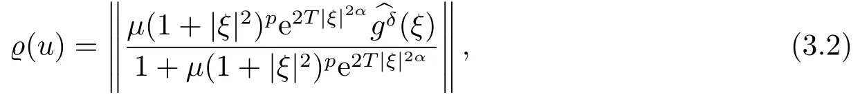
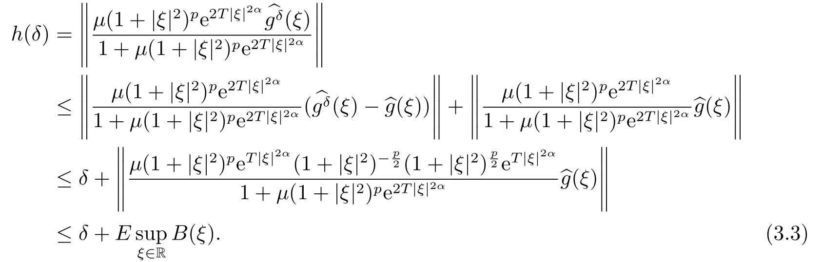
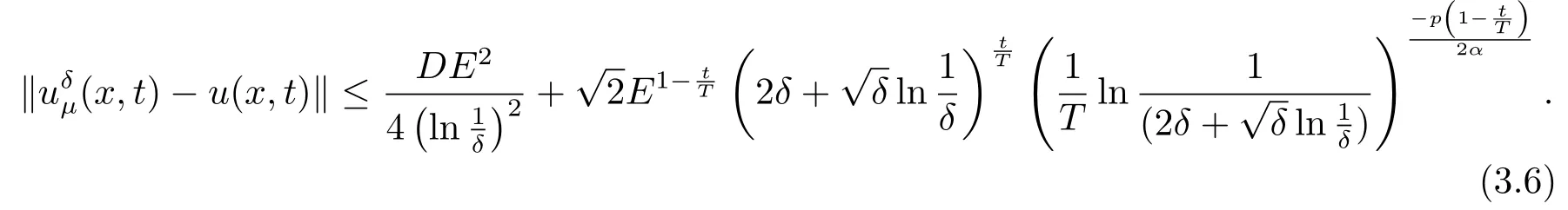
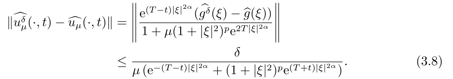
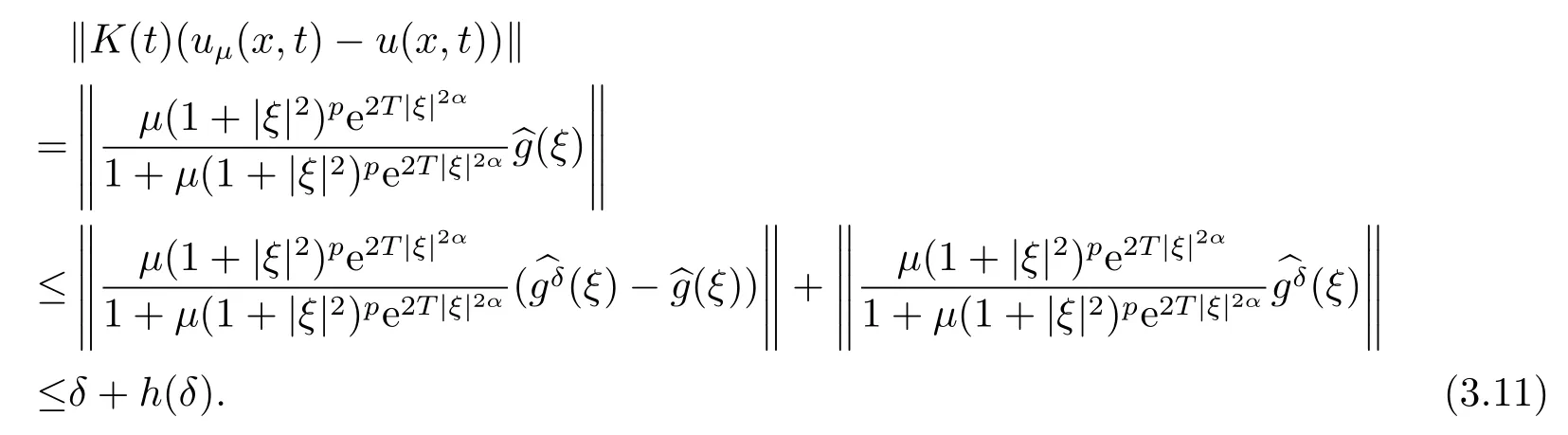
3.A-posteriori Convergence Estimate


4.Numerical Simulations