
LARGE-TIME BEHAVIOR OF SOLUTIONS TO THE INFLOW PROBLEM OF THE NON-ISENTROPIC MICROPOLAR FLUID MODEL?
2021-09-06 07:54:36高俊培崔海波
(高俊培) (崔海波)
School of Mathematical Sciences,Huaqiao University,Quanzhou 362021,China E-mail:hbcui@hqu.edu.cn
Abstract We investigate the asymptotic behavior of solutions to the initial boundary value problem for the micropolar fluid model in a half line R+:=(0,∞).Inspired by the relationship between a micropolar fluid model and Navier-Stokes equations,we prove that the composite wave consisting of the transonic boundary layer solution,the 1-rarefaction wave,the viscous 2-contact wave and the 3-rarefaction wave for the in flow problem on the micropolar fluid model is time-asymptotically stable under some smallness conditions.Meanwhile,we obtain the global existence of solutions based on the basic energy method.
Key words Micropolar fluid model;composite wave;in flow problem;stability
1 Introduction
The 1-D compressible viscous micropolar fluid model in the half line R=:(0,
+∞)reads as follows,in Eulerian coordinates:
ρ
,u
,ω
andθ
represent the mass density,velocity,microrotation velocity and temperature of the fluid,respectively.We assume that A,μ
,κ
are positive constants.Assuming that the fluid is perfect and polytropic,for pressurep
and internal energye
we have the state equations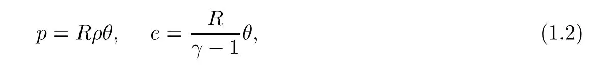
R
andγ>
1 are positive constants.We consider the system(1.1)with the initial values

x
=+∞is constant,namely,that
ρ
,u
,ω
andθ
atx
=0 are given by
ρ
>
0,u
>
0,θ
>
0,ω
are constants,and the following compatibility conditions hold:
The boundary conditions for the half-place problem(1.1)can be proposed as one of the following three cases:
Case 1.Out flow problem(negative velocity on the boundary):

Case 2.Impermeable wall problem(zero velocity on the boundary):

Case 3.In flow problem(positive velocity on the boundary):

ρ
could not be given,but in Case 3,ρ
must be imposed due to the well-posedness theory of the hyperbolic equation(1.1).
ω
=0 for the large time behavior of solutions to the initial boundary value problem(1.1),(1.3),(1.4),(1.5)and(1.6),then the micropolar fluid model(1.1)can be reduced to the following single Navier-Stokes system:
Moreover,when the dissipation effects are neglected for the large time behavior,Navier-Stokes system(1.10)can be reduced to the following Euler system:
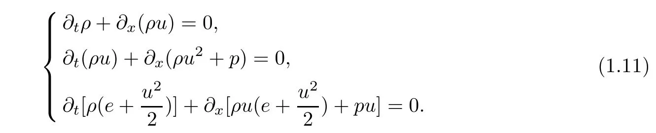
It is well known that Euler system(1.11)is a typical example of the hyperbolic conservation laws.The Riemann solutions for Euler system(1.11)contain three basic wave patterns–two nonlinear waves,called a shock wave and a rarefaction wave,and one linear wave,called contact discontinuity and their linear combinations.Later,not only basic wave patterns but also a new wave,which is called a boundary layer solution(BL-solution for brevity)[20],may appear in the initial boundary value problem,because the large time behavior of solutions to the Cauchy problem(on the isentropic or nonisentropic Navier-Stokes system)are basically described by the viscous versions of three basic wave patterns.There have been a lot of mathematical studies about basic wave patterns and the BL-solution to the isentropic or nonisentropic Navier-Stokes system;for more on these,please refer to[8–12,14,18,20–22,28,29,31].
Now we review some recent work on the in flow and out flow problems of the micropolar fluid model.Yin[5,35]obtained the stability of the BL-solution to the in flow and out flow problems.In a previous paper[35],Yin proved the stability of the composite wave consisting of the subsonic BL-solution,the viscous 2-contact wave,and the 3-rarefaction wave under the condition that the amplitude of the contact wave and the BL-solution is small enough but the 3-rarefaction wave is not necessarily small enough for the one dimensional compressible micropolar fluid model.
This brings us to a natural question:Can we obtain the asymptotic stability of the composite wave,consisting of the transonic BL-solution,the 1-rarefaction wave,the viscous 2-contact wave and the 3-rarefaction wave,for the in flow problem on micropolar fluid model(1.1)of the Riemann problem on Euler system(1.11)in the setting ofω
(x,t
)=0 under the condition thatω
=0?We will give a positive answer to this question in this paper.As far as we know,this is the first work on the stability of a composite wave of the transonic BL-solution,the 1-rarefaction wave,the viscous 2-contact wave and 3-rarefaction wave for the compressible micropolar fluid model.It is worthwhile pointing out that the four wave patterns are different from the Cauchy problem due to the boundary effect.Correspondingly,some new mathematical difficulties occur due to the degeneracy of the transonic BL-solution and its interactions with other wave patterns in the composite wave.In order to study the large time behavior of solutions to(1.1),(1.3),(1.4),(1.5)and(1.6),it is convenient to use the following Lagrangian coordinate transformation:

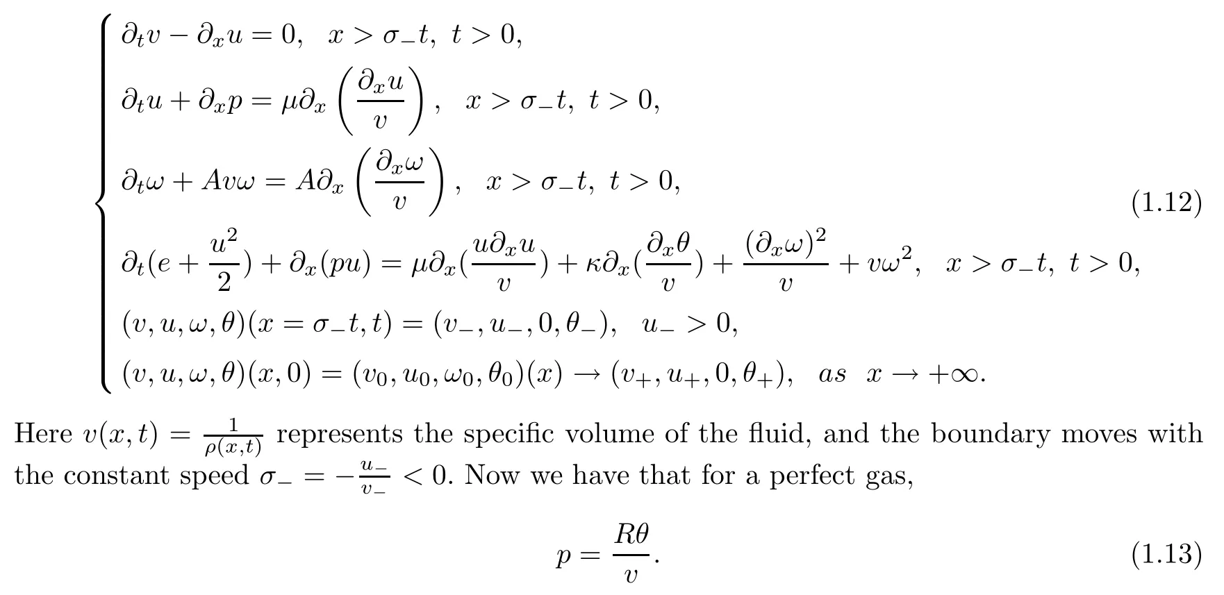
The system(1.1)can be transformed into the following moving boundary problem of a micropolar fluid model in the Lagrangian coordinates:
x
=σ
t
,we introduce a new variable,ξ
=x
?σ
t
.Then we have the half-space problem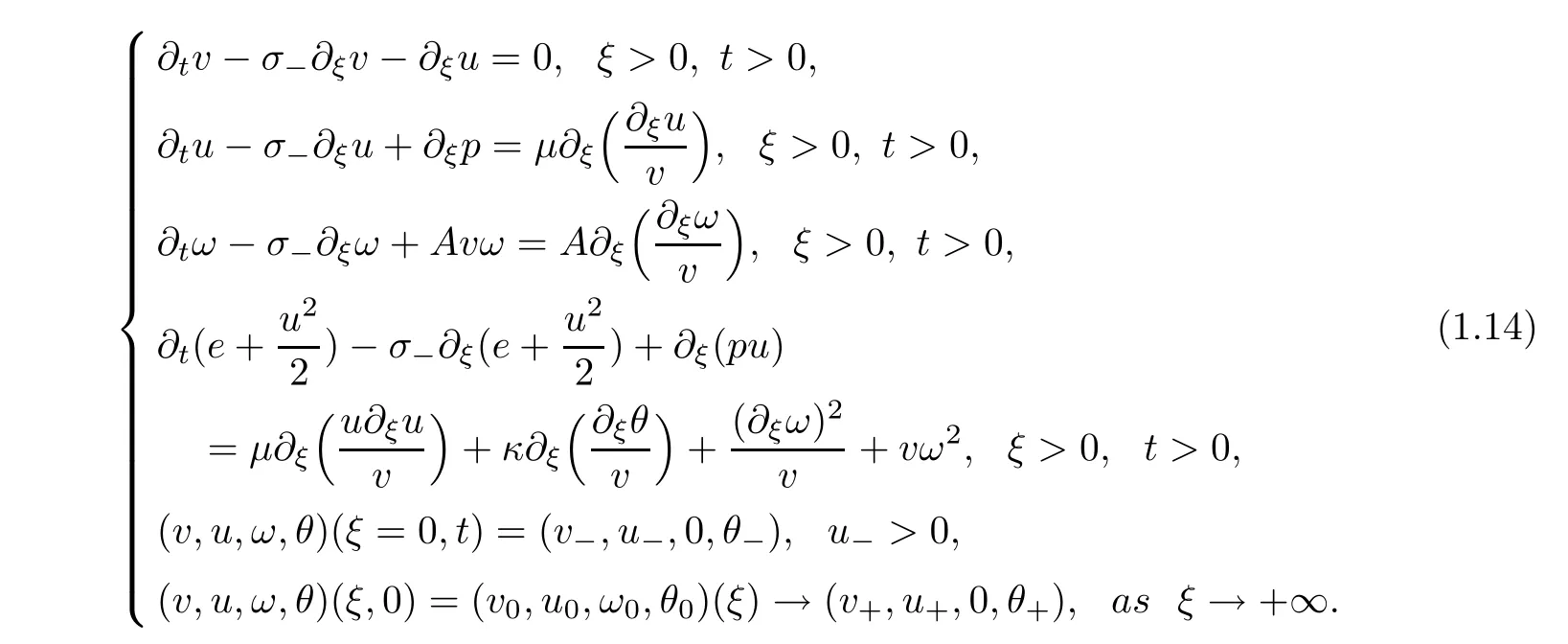
v,p,e
,the temperatureθ
(>
0)and entropys
,the remaining three variables can be expressed.Without loss of generality,we de fine the entropys
as
which obeys the second law of thermodynamics,namely,that

s
(v
(x
),θ
(x
))is expressed by(v
(x
),θ
(x
))as follows: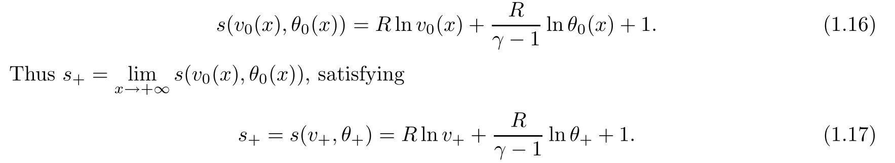
The rest of the paper is arranged as follows:in Section 2,we give some preliminaries of the Navier-Stokes system,then we reformulate the original system(1.1)and introduce our main theorem concerning the global existence and asymptotic stability of solutions.The proof of Theorem 2.4 is concluded in Section 3.In Appendix,we present the details of some proofs,for completeness of the paper.
2 Some Preliminaries of the Navier-Stokes System
Since we expect the large time behavior of micropolar fluid model(1.14)to be the same as that of the Navier-Stokes system,we assume thatω
(x,t
)=0 for the large time behavior.Therefore,when timet
→+∞,the micropolar fluid models(1.12)and(1.14)become the Navier-Stokes systems: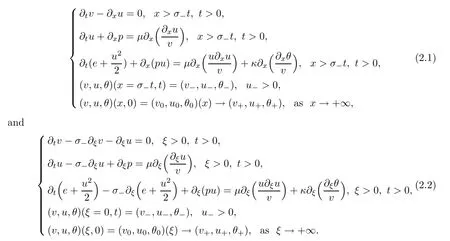
v
,u
,θ
)belonged to the subsonic,transonic,and supersonic regions,and proved the asymptotic stability of not only the single contact wave but also the composite wave consisting of the subsonic BL-solution,the contact wave,and the rarefaction wave.Now,in order to prove that the composite wave consisting of the transonic BL-solution,the 1-rarefaction wave,the viscous 2-contact wave,and the 3-rarefaction wave for the in flow problem on the micropolar fluid model(1.14)is time-asymptotically stable,we first review some known results about the Navier-Stokes system in[32]which will be used repeatedly in this paper.For any given right state(v
,u
,θ
),we can de fine wave curves(BL-solution curve,1-rarefaction wave curve,viscous 2-contact wave curve and 3-rarefaction wave curve)in terms of(v,u,θ
)withv>
0 andθ>
0 in the phase space as follows:*Transonic boundary layer curve:
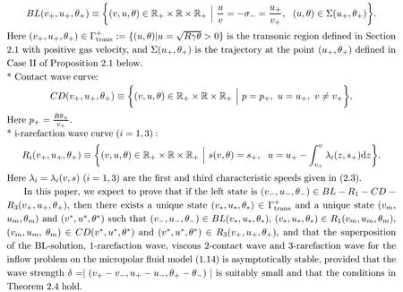
2.1 BL-solutions
The characteristic speeds of the hyperbolic part of(2.1)are
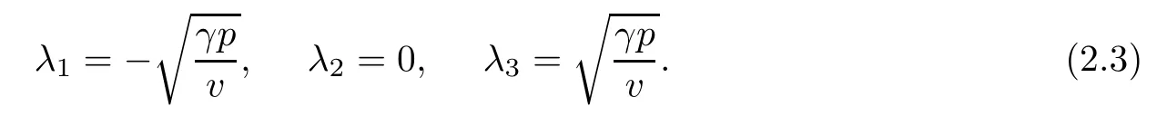
The first and third characteristic fields are genuinely nonlinear,and may have nonlinear waves,shock waves and rarefaction waves,while the second characteristic field is linearly degenerate,and here contact discontinuity may occur(See[34]).
The sound speedC
(v,θ
)and the Mach numberM
(v,u,θ
)are de fined by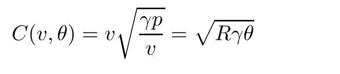

V
,U
,
Θ)(ξ
)satis fies the ODE system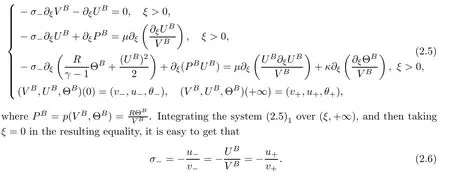
Then the existence and uniqueness for the ODE system(2.5)are given as follows(for later use,we only list some useful properties of solutions for(2.5)):
Proposition 2.1
(See[31])Assume thatv
>
0,u
>
0 andθ
>
0,and de fineδ
=|(u
?u
,θ
?θ
)|.Ifu
≤0,then there is no solution to(2.5).Ifu
>
0,then there exists a suitable small constantδ
>
0 such that,if 0<δ
≤δ
,then we have the following cases:Case I.Supersonic case:M
>
1.Then there is no solution to(2.5).Case II.Transonic case:M
=1.Then there exists a unique trajectory Σ tangential to the line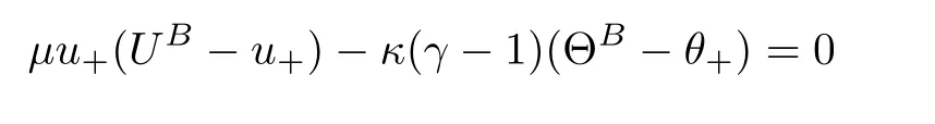
u
,θ
).For each(u
,θ
)∈Σ(u
,θ
),there exists a unique solution(U
,
Θ)satisfying
M
<
1.Then there exists a center-stable manifold M tangential to the line
u
,θ
),wherea
andc
are some positive constants(see[31]for their de finitions).Only when(u
,θ
)∈M(u
,θ
)does there exist a unique solution(U
,
Θ)?M(u
,θ
)satisfying
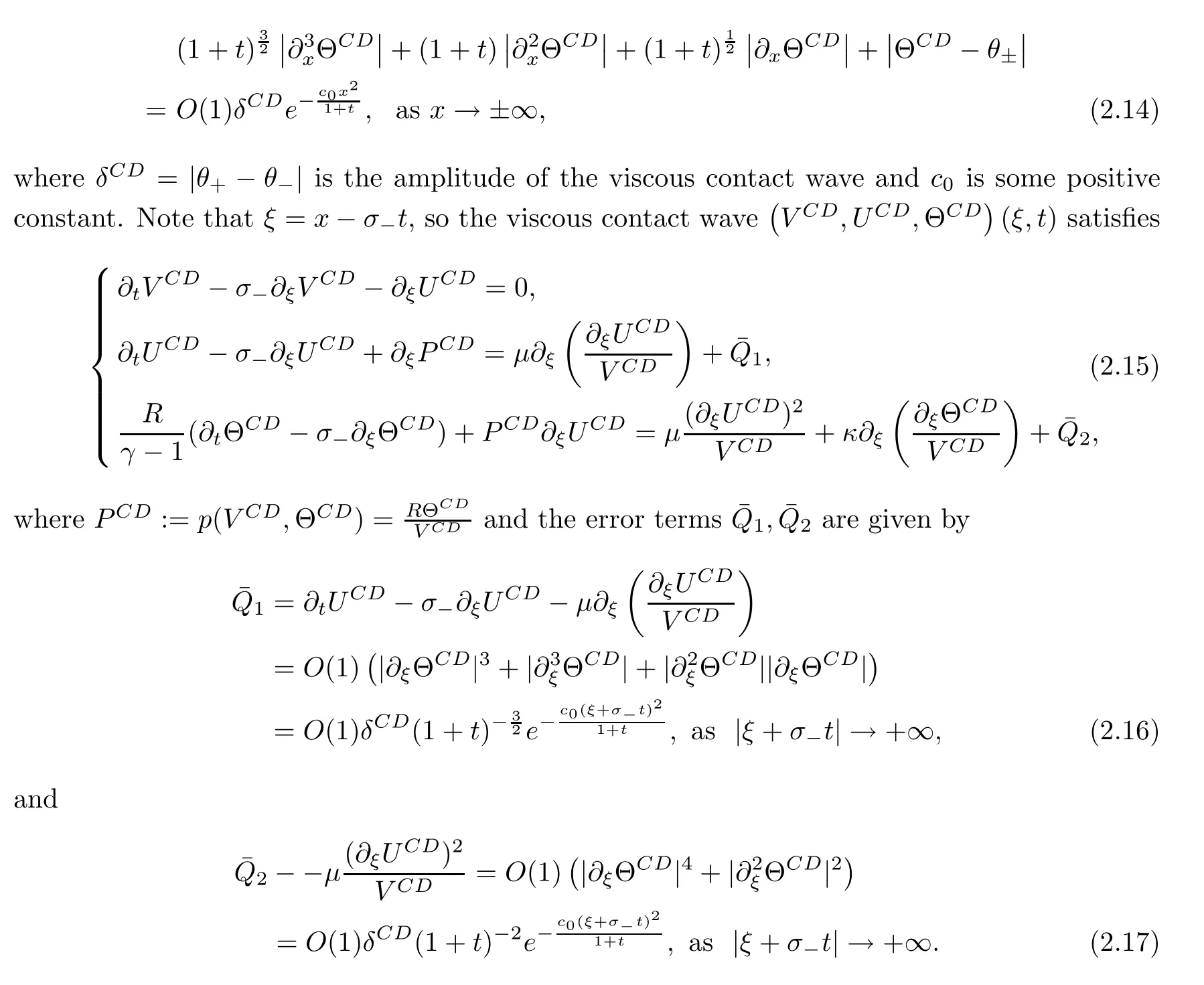
2.2 Viscous contact wave
If(v
,u
,θ
)∈CD
(v
,u
,θ
),that is,
then the Riemann problem of the Euler system
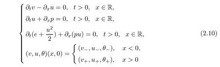
admits a single contact discontinuity solution

Thus the viscous contact wave de fined in(2.13)satis fies the property
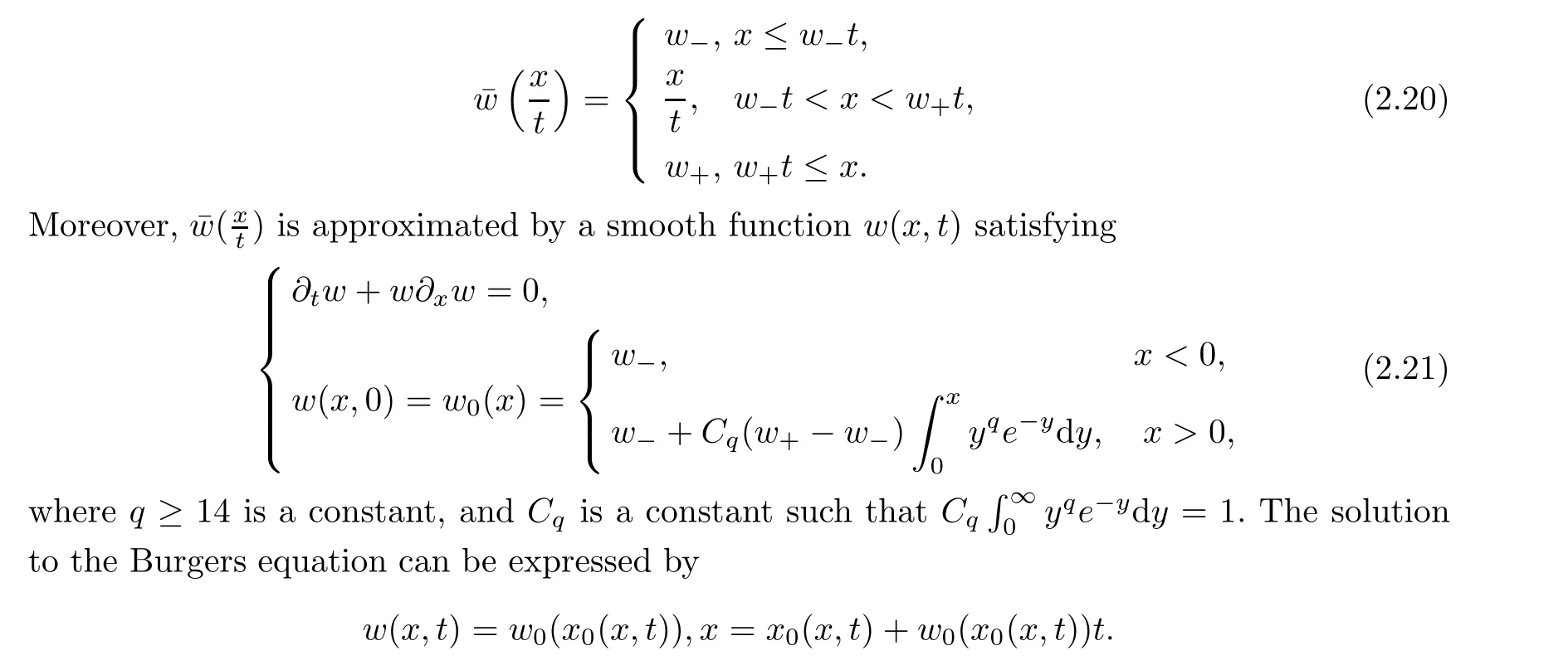
2.3 Rarefaction wave
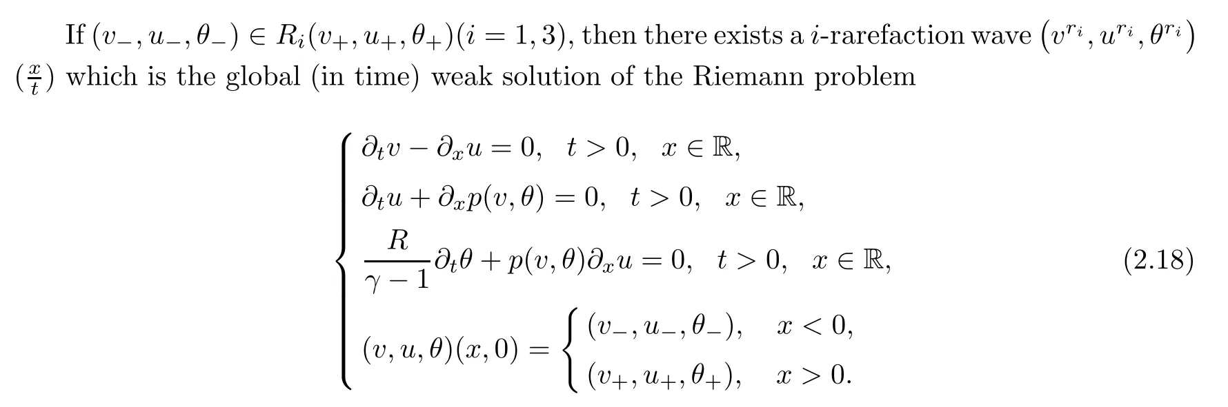
w
<w
,the following Riemann problem on the Burgers equation:

σ
>
0 and forx
≥0,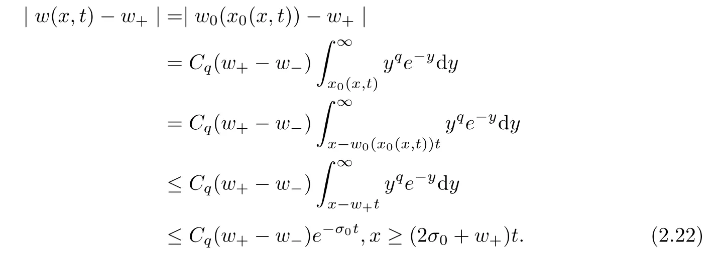
w
(x,t
)of the Burgers equation(2.21)has the following properties:Lemma 2.2
Letting 0<w
<w
,δ
:=w
?w
,Burgers equation(2.21)has a unique smooth solutionw
(x,t
)which satis fies the following properties:(i)w
≤w
(x,t
)<w
,?
w
≥0 forx
∈R andt
≥0;(ii)for anyp
(1≤p
≤∞),there exists a positive constantC
such that,fort
≥0,
ξ
=x
?σ
t
,so the smoothed i-rarefaction wave(V
,U
,
Θ)(ξ,t
)(i
=1,
3)de fined above satis fies
2.4 Composite waves and main results
De fine the composite wave(V,U,
Θ)(ξ,t
)by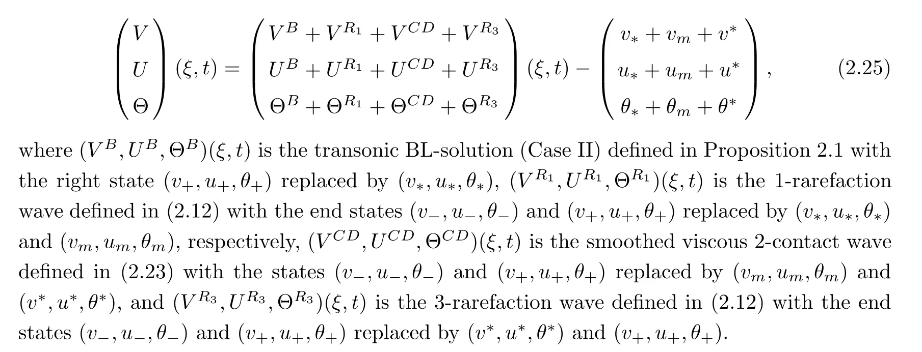
Now we state the main result of our paper.
Theorem 2.4
For any given[v
,u
,ω
,θ
]withv
>
0,u
>
0 andθ
>
0,we suppose thatu
>
0,ω
=0 and(v
,u
,θ
)∈BL
?R
?CD
?R
(v
,u
,θ
).Let[V,U,
Θ](ξ,t
)be the composite wave consisting of the transonic BL-solution,the 1-rarefaction wave,the viscous 2-contact wave,and the 3-rarefaction wave de fined in(2.25).There exist positive constantsδ
>
0 andC
>
0 such that if
δ
=|(v
?v
,u
?u
,θ
?θ
)|satisfy
v,u,ω,θ
](ξ,t
)satisfying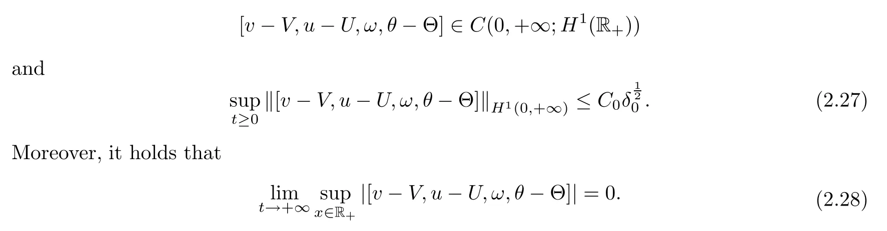
Remark 2.5
In Theorem 2.4,we assume thatδ
=|(v
?v
,u
?u
,θ
?θ
)|is suitably small.This assumption is equivalent to stating that the amplitudes of the four waves are all suitably small.Remark 2.6
This model can also be generalized to general gases.3 Global Existence and Large Time Behavior
3.1 Wave interaction estimates
From(2.5),(2.15),(2.24)and(2.25),by a careful calculation,we have

In order to control the interaction terms coming from different wave patterns,we give the following lemma,which will be important in the energy estimate:
Lemma 3.1
(Wave interaction estimates[32])
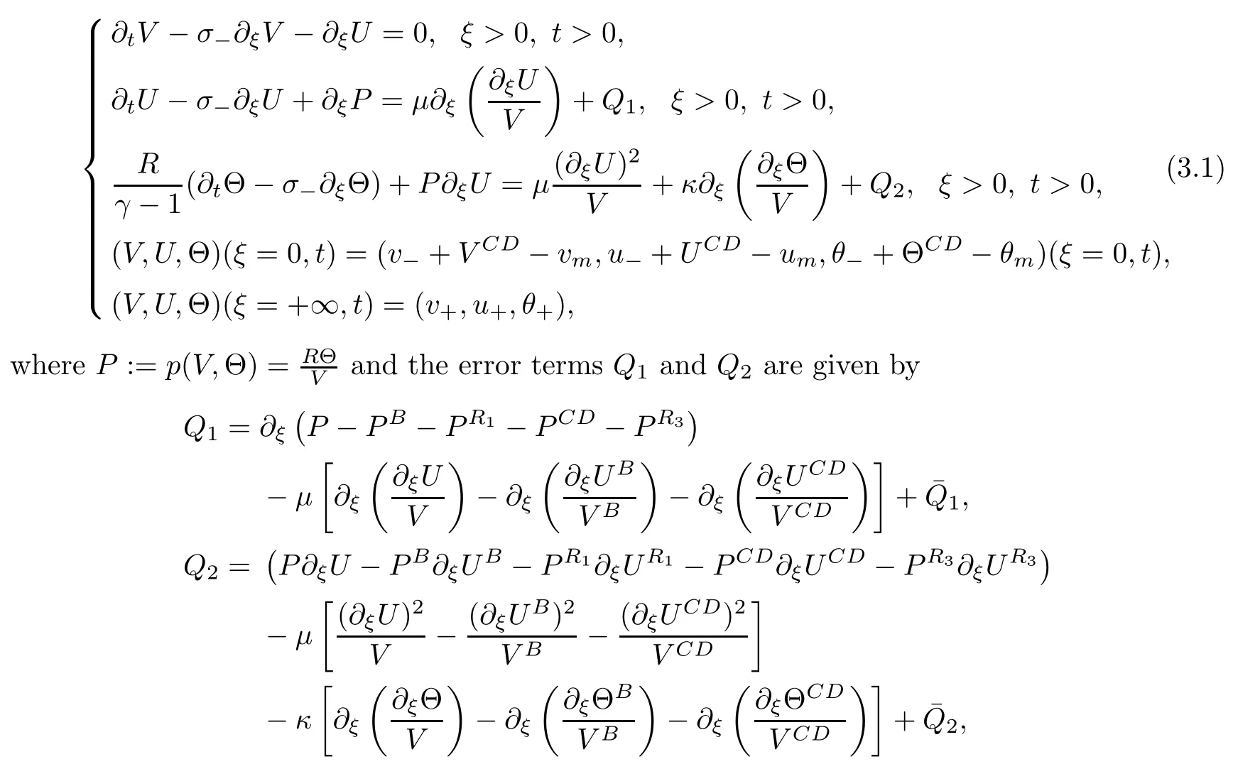
3.2 Reformulation of the problem
We first de fine the perturbation as

?,ψ,ω,ζ
](ξ,t
)satis fies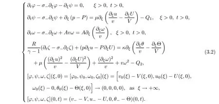
The key to the proof of the global existence part of Theorem 2.4 is to derive the uniform a priori estimates of solutions to the half-space problem(3.2).Our a priori assumption is de fined as follows:

ε
is a small positive constant.Proposition 3.2
(A priori estimates)Assume that all of the conditions listed in Theorem 2.4 hold.Let[?,ψ,ω,ζ
](ξ,t
)be a solution to the half-space problem(3.2)on 0≤t
≤T
for some positive constant T.There are constantsδ
>
0 andC>
0 such that if[?,ψ,ω,ζ
]∈C
(0,T
;H
(R))and
t
∈[0,T
],the solution[?,ψ,ω,ζ
](ξ,t
)satis fies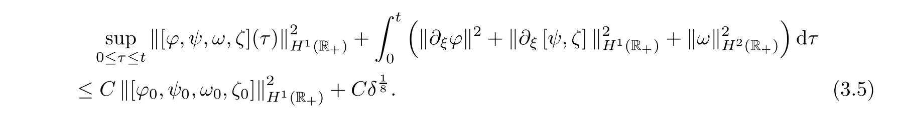
From a priori assumption(3.3),it is easy to get that

where the Sobolev inequality

is used.
3.3 Energy estimates
Lemma 3.3
(Boundary estimates[31])There exists a positive constant C such that,for anyt>
0,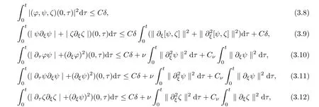
ν
is a positive small constant to be determined later,andC
is a positive constant depending onν
.Lemma 3.4
Assuming that the conditions in Proposition 3.
2 hold,we have the following energy estimate fort
∈[0,T
]: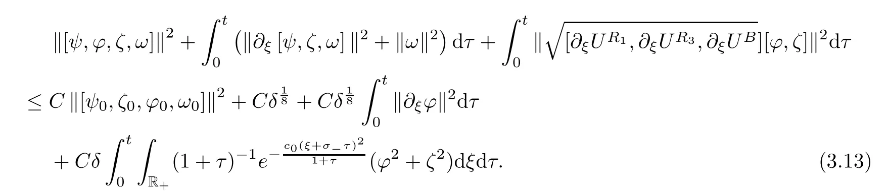
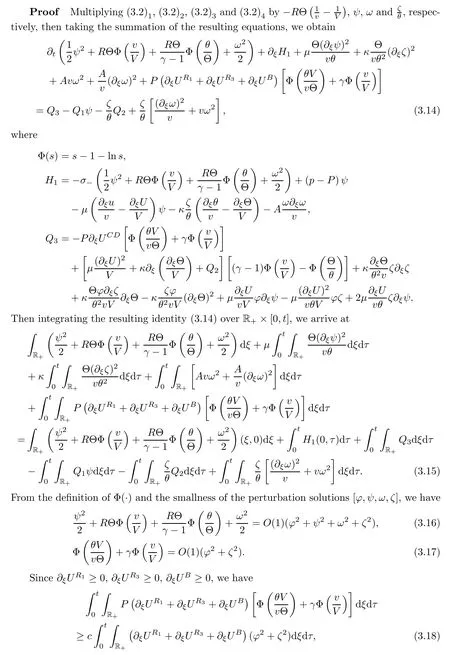
where we have used(3.17).
By applying the a priori assumption(3.3),(3.2),(2.16),(2.17),Cauchy-Schwarz’s inequality with 0<ν<
1,(3.16),(3.17)and(3.6),Sobolev’s inequality(3.7)and Lemma 3.3,we obtain the estimates for the right hand side of(3.15)as follows: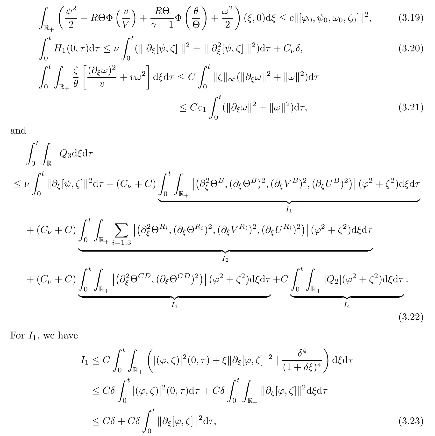
where we have used(2.7),(3.8)and the fact that

From the properties of the viscous 2-contact wave,we can get that

I
,we have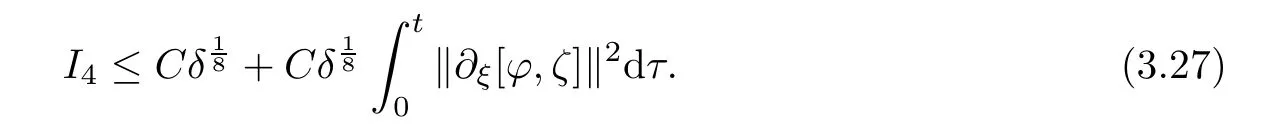
Thus,substituting(3.23)–(3.27)into(3.22),we have
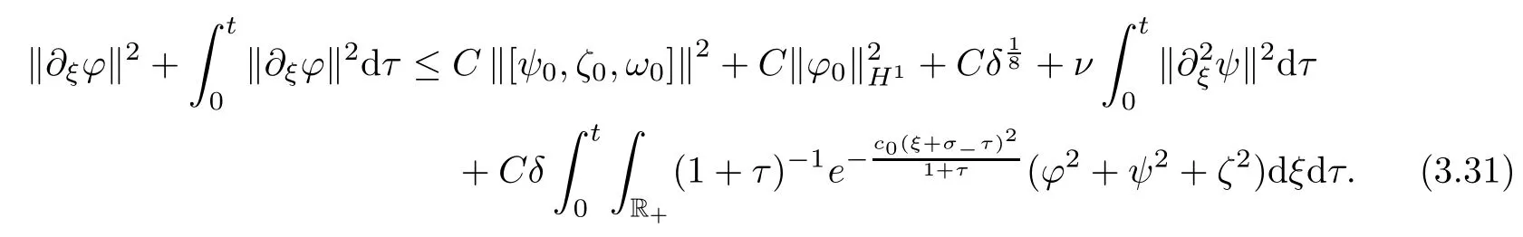
Now we estimate the last two terms as follows:

ν
andδ
be suitably small,we obtain(3.13),and thus complete the proof of Lemma 3.4.Lemma 3.5
Assume that the conditions in Proposition 3.
2 hold.Then we have the following energy estimate fort
∈[0,T
]:
Proof
We first differentiate(3.2)with respect toξ
,and then obtain
v?
?
andμ?
?
,respectively,and integrating the resulting equalities over R×[0,t
],one has
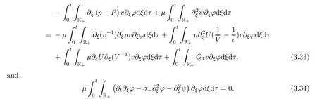
The summation of(3.33)and(3.34)further implies that
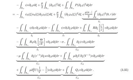
<ν<
1,Sobolev’s inequality(3.7),and Lemma 3.3,we can estimateI
(5≤i
≤14)as follows:

I
(5≤i
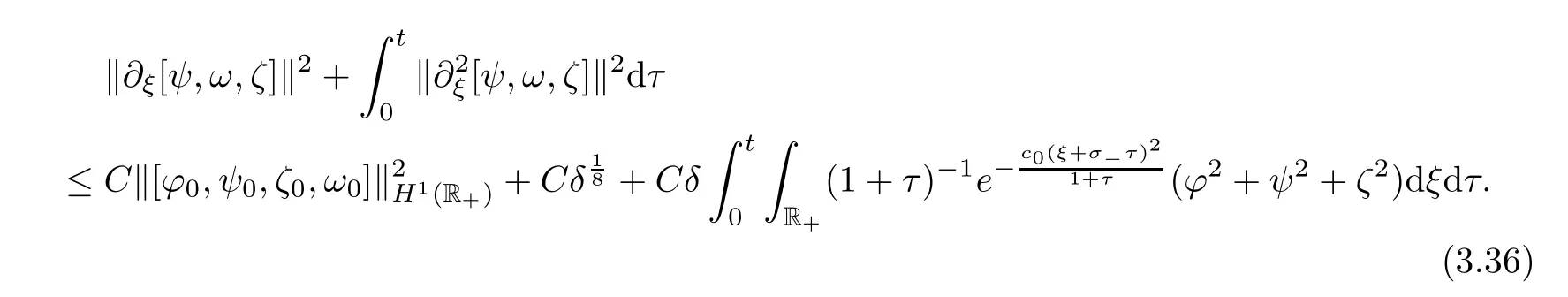
≤14)and(3.13)into(3.35),lettingν,δ
andε
be suitably small,and using Cauchy-Schwarz’s inequality,we obtain(3.31).Thus we complete the proof of Lemma 3.5.Lemma 3.6
Assume that the conditions in Proposition 3.
2 hold.Then we have the following energy estimate fort
∈[0,T
]:

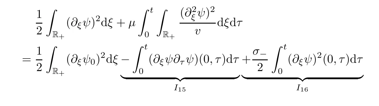
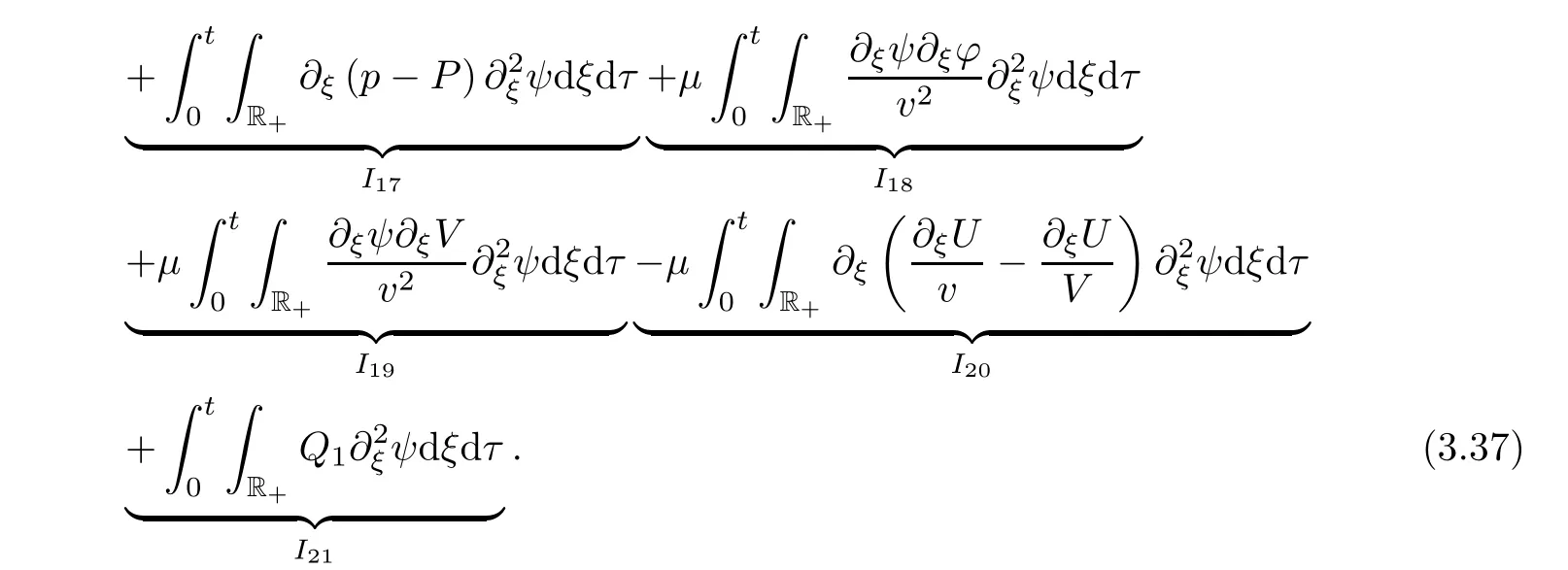
I
(15≤i
≤21)term by term.For brevity,we directly give the following computations: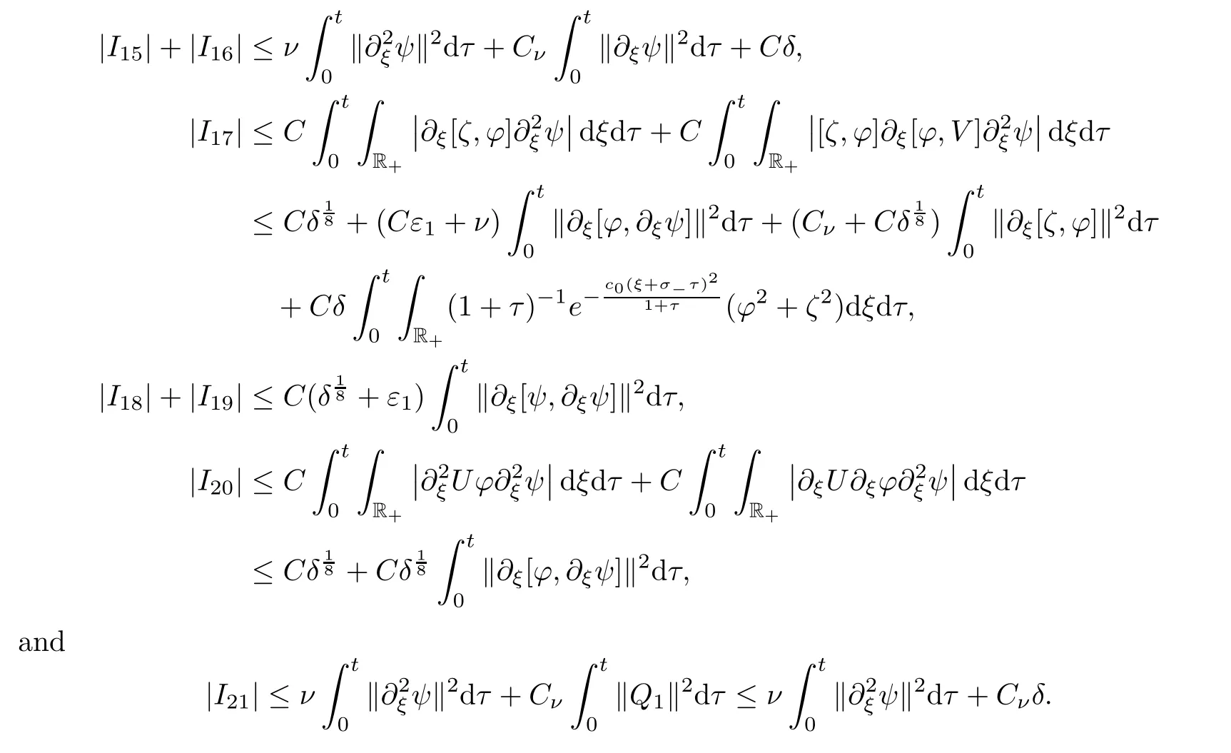
I
(15≤i
≤21)into(3.37),and recalling(3.31)and(3.13),we then chooseδ>
0 andν>
0 suitably small in order to derive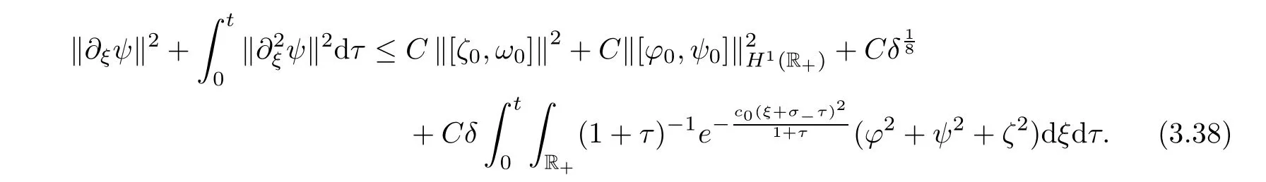


σ
<
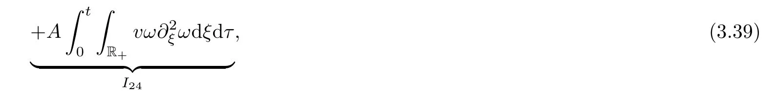
0 to deal with the boundary term.To obtain the estimates forI
(22≤i
≤24),we use Cauchy-Schwarz’s inequality with 0<ν<
1,Sobolev’s inequlity(3.7),and the a priori assumption(3.3)to obtain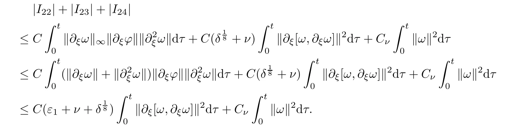
ε
>
0,δ>
0 andν>
0 suitably small to derive
Summing up(3.41),(3.40)and(3.38),we get the desired estimate,(3.36).Thus we have completed the proof of Lemma 3.6.
Proof of Proposition 3.2
Now,we are ready to prove Proposition 3.2.Combining Lemmas 3.4-3.6 with Lemma 4.2 in the Appendix,and if the wave strengthδ
and the constantsε
are small enough,then for allt
∈[0,T
],we have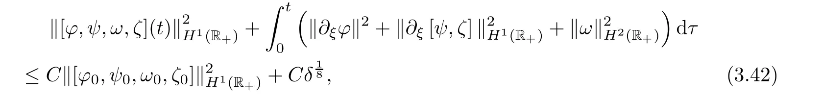
.
Proof of Theorem 2.4
We are now in a position to complete the proof of Theorem 2.4.In view of the energy estimates obtained in Proposition 3.2,one sees that
δ
are parameters independent ofε
.By lettingδ
be small enough,the global existence of the solution of the half-space problem(3.2)then follows from the standard continuation argument based on the local existence and the a priori estimate(3.5).Moreover,(3.43)and(2.26)imply(2.27).Our next intention is to prove the large time behavior for(2.28).For this,we first justify the following limits:
To prove(3.44),we get from(3.2),(3.5),(2.14),Lemma 2.3 and(2.8)that
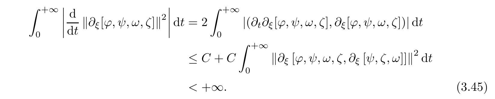
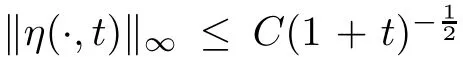
Consequently,(3.45),together with(3.5),gives(3.44).Then(2.28)follows from(3.44)and Sobolev’s inequality(3.7).This ends the proof of Theorem 2.4.
4 Appendix
In this appendix,we will give some basic results used in the paper.Lemma 4.1 and Lemma 4.2 are borrowed from[10]and[31],and we omit some details here.
Lemma 4.1
Suppose thath
(ξ,t
)satis fies
Then the following estimate holds:

α>
0 is a constant to be determined later.We now give some estimates concerning the delicate term
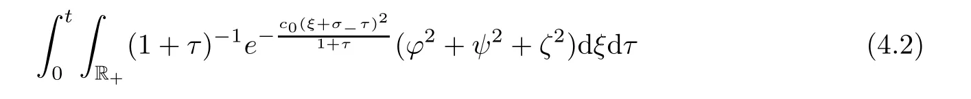
by using Lemma 4.1.
Lemma 4.2
Under the conditions of Proposition 3.2,there exists a constantC>
0 such that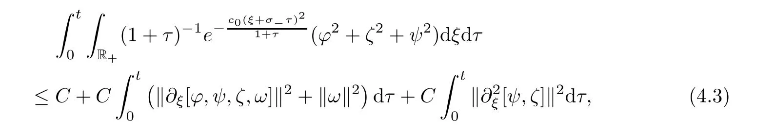
δ
is small enough.Proof
For anyν>
0,the proof of inequality(4.3)consists of the following two parts:
γ
?1 and adding the resulting inequality to(4.5)and takingδ
suitably small easily implies(4.3).We first prove(4.4).De fine

We then rewrite(3.2)as follows:

Rζ
?P?
)vη
and integrating the resulting equation over R×[0,t
]leads to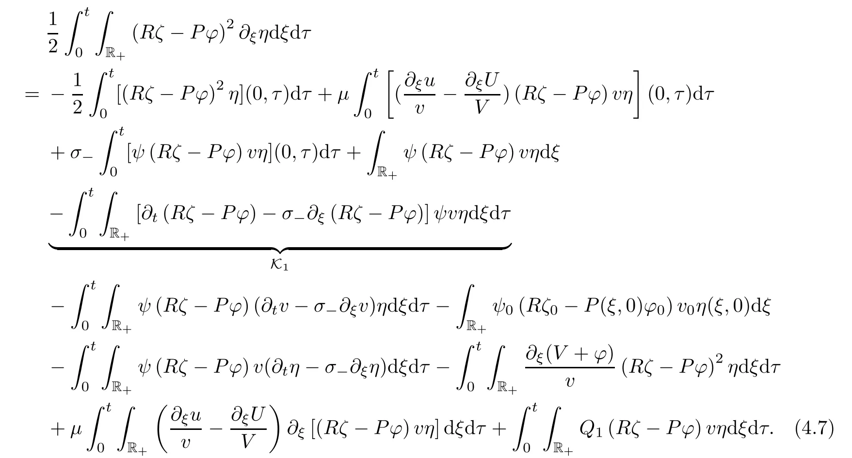
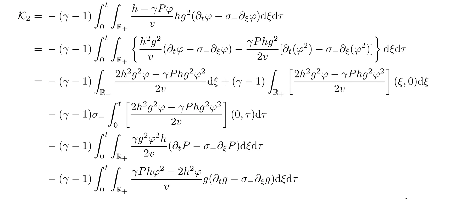
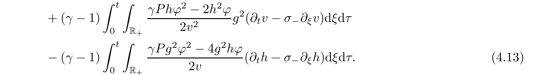
The delicate term Kcan be rewritten as


where in the second identity we have used(3.2)and(3.2).Since

by combining(4.7)and(4.8),we have
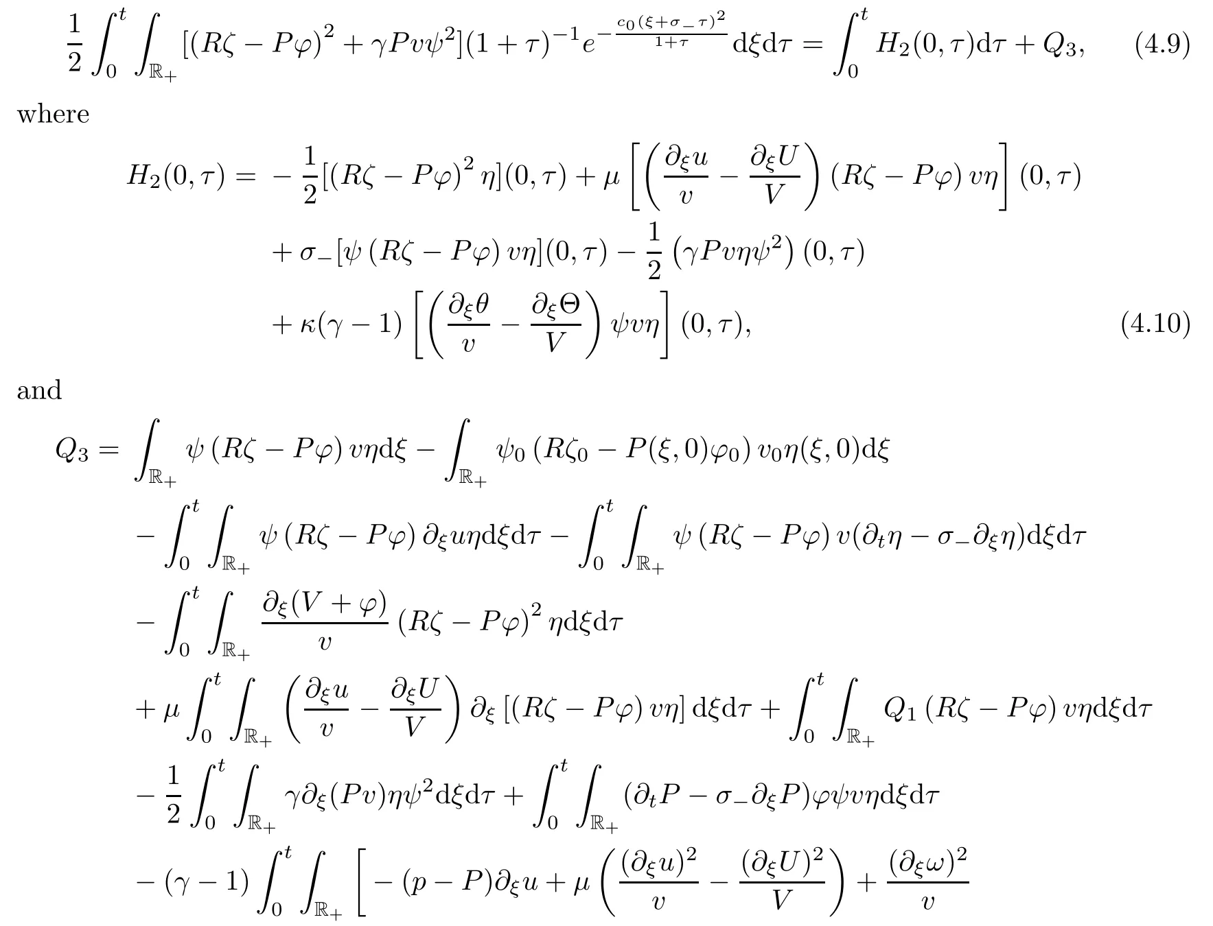

From Lemma 3.3(boundary estimates),we have

h
=Rζ
+(γ
?1)P?
.Then from(3.2)and(3.2),we have

Acknowledgements
Cui would like to thank Prof.Changjiang Zhu and Dr.Haiyan Yin for his continuous encouragement. Acta Mathematica Scientia(English Series)2021年4期
- Acta Mathematica Scientia(English Series)的其它文章
- REGULARITY OF WEAK SOLUTIONS TO A CLASS OF NONLINEAR PROBLEM?
- EXISTENCE TO FRACTIONAL CRITICAL EQUATION WITH HARDY-LITTLEWOOD-SOBOLEV NONLINEARITIES?
- A DIFFUSIVE SVEIR EPIDEMIC MODEL WITH TIME DELAY AND GENERAL INCIDENCE?
- ON A COUPLED INTEGRO-DIFFERENTIAL SYSTEM INVOLVING MIXED FRACTIONAL DERIVATIVES AND INTEGRALS OF DIFFERENT ORDERS?
- CLASSIFICATION OF SOLUTIONS TO HIGHER FRACTIONAL ORDER SYSTEMS?
- ENERGY CONSERVATION FOR SOLUTIONS OF INCOMPRESSIBLE VISCOELASTIC FLUIDS?