
REGULARITY OF WEAK SOLUTIONS TO A CLASS OF NONLINEAR PROBLEM?
2021-11-13 01:11:15周建豐
(周建豐)
School of Mathematical Sciences,Peking University,Beijing 100871,China E-mail:jianfengzhou xmu@163.com
Zhong TAN (譚忠)
School of Mathematical Sciences,Xiamen University,Xiamen 361005,China E-mail:ztan85@163.com
Abstract We study the regularity of weak solutions to a class of second order parabolic system under only the assumption of continuous coefficients.We prove that the weak solution u to such system is locally Hlder continuous with any exponent α∈(0,1)outside a singular set with zero parabolic measure.In particular,we prove that the regularity point in QTis an open set with full measure,and we obtain a general criterion for the weak solution to be regular in the neighborhood of a given point.Finally,we deduce the fractional time and fractional space differentiability of Du,and at this stage,we obtain the Hausdorff dimension of a singular set of u.
Key words Parabolic system;regularity;weak solution;Hausdorff dimension
1 Introduction
Letting ??Rn(n≥2)be a bounded domain,we aim in this paper to study the regularity of a weak solution to the inhomogeneous parabolic system

withz=(x,t)∈?×(?T,0)≡QT,andT>0.a(·):QT×RN×RNn→RNn,u:QT→RN,b:QT×RN×RNn→RN,N∈Z+,N≥1.In general,the solution of parabolic system(1.1)cannot be expected to be regular everywhere on the domain,even the homogeneous case
It is worth noting that everywhere regularity can be obtained only with a special structure ona(z,u,Du),such as the evolutionaryp?Laplacian system
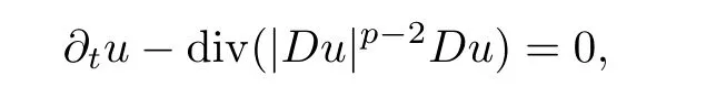
for which the regularity problem was settled by the fundamental contributions of Dibenedetto and Friedman[19–21],otherwise it fails in general(see[44–46],for example).
One can,however,expect partial regularity results;this is regularity away from a singular set that is in some sense small.The partial regularity for general parabolic(1.2)was a longstanding open problem until it was solved by Duzaar and Mingione[28],Duzaar,Mingione and Steffen[29],C.Scheven[40]and also Duzaar et al.[8,9,25];their proofs are based on theAcaloric approximation method to the parabolic setting.Subsequently,Scheven[40]derived an analogous result for the subquadratic case of(1.2).Moreover,Baroni[3]showed the continuity of the gradientDuwhile only assuming the Dini continuity ofa(·,·,Du).Under the assumption of continuous coefficients,Bgelein-Foss-Mingione[11]proved partial Hlder continuity results for(1.2)with polynomial growth.When considering the boundary regularity of the parabolic system,the same authors[8,9]showed that almost every parabolic boundary point is a Hlder continuity point forDu.There have been many research articles on the regularity of weak solutions to parabolic system,for example,[1,12,34,39,47]and the reference therein.
The above results for parabolic problems are analogous to results for the elliptic case(see[37]),the application of the so called harmonic approximation to prove regularity theorems goes back to Simon[41,43]and Duzaar et al.[26,27].In terms of related results for problems with continuous coefficients,Campanato[17](see also[16])derived the Hlder continuity of the solutions of some nonlinear elliptic system in R.For higher dimension cases,Foss-Mingione[31]proved the partial Hlder continuity for solutions to the elliptic system,and the proof relies upon an iteration scheme of a decay estimate for a new type of excess functional measuring the oscillations in the solution and its gradient.Afterwards,Beck[4]showed the boundary regularity of the elliptic system with a Dirichlet condition.When considering the Dini continuous coefficients,Duzzar-Gastel[24]presented a general low-order partial regularity theory.In particular,for the system with variable exponentp(x),Habermann[33](see also[2])derived the partial Hlder continuity for a weak solution to a nonlinear problem with a continuous growth exponent.For more details,one can also refer to[5,7,22,30,32,35,48,50]and the reference therein.
Turning to the technically more challenging case of(1.1),as far as we are aware,there has been no previous work addressing the partial regularity of a weak solutionuto(1.1)with continuous coefficients(cf.[11]for the homogeneous case(1.2)).Thus,in the present paper,we aim to fill a gap in the partial regularity theory of the quasi-linear parabolic system(1.1).This turns out to be a difficult task,since the inhomogeneous termb(z,u,Du)will lead to several new difficulties:
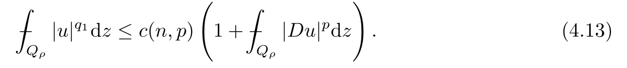
1.When establishing the Poincarinequality in Section 4,we are not able to obtain(4.13)directly,due to the lack of a zero-boundary condition ofuon?Bρfor anyBρ??.In order to avoid this flaw,a iteration argument will be needed;
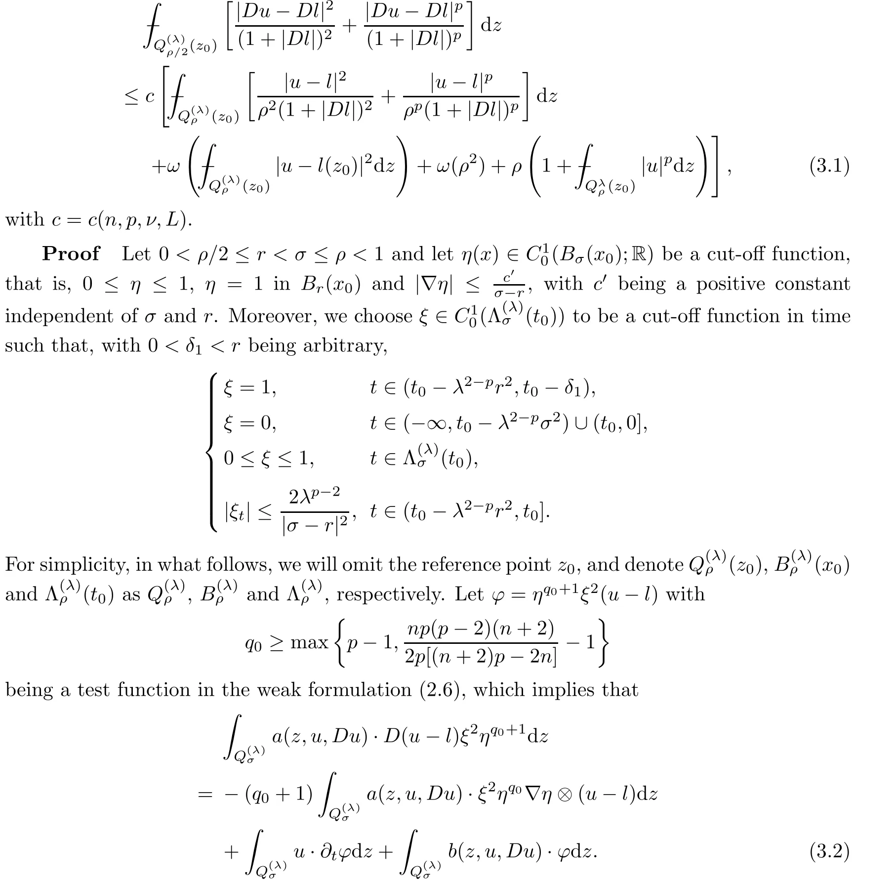
2.For proving Caccioppoli’s inequality(3.1),the key point is boundingb(z,u,Du)in terms ofDu?Dloru?l(lis an affine function,which will be de fined in later).However,one cannot use the inequalityl(z)≤l(z0)+Dl≤Mdirectly for a.e.z∈Qρ,ρ≤1 withM≥1 being a constant;otherwise,the constant after(5.12)would depend onMwithM=Hλ(see(5.7)and(Aj)).As a consequence,all constants in Lemma 5.3 depend onλso that the estimates could blow up during the iteration process.At this stage,we shall use a weighted Sobolev interpolation inequality(see[6,13]).For a suitable functionw(·):??→R+satis fing
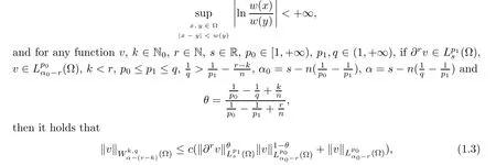
wherecdepends onp0,p1,n,q,r,k.Here,we have de fined
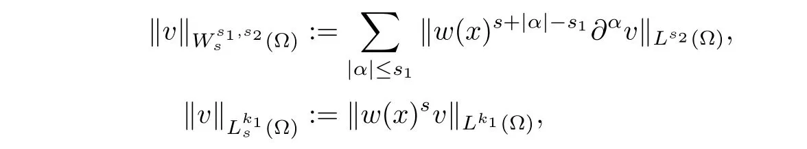
withs1∈N,k1,s2≥1 ands∈R.
The main result of this paper is as follows:
Theorem 1.1Letp≥2 andu∈C0(?T,0;L2(?;RN))∩Lp(?T,0;W1,p(?;RN))be a weak solution of the parabolic system(1.1)inQTunder the assumptions(2.1)–(2.5).Then,there exists an open subsetQ0?QTsuch that

for everyα∈(0,1).Moreover,we have the singular set satis fingQTQ0?Σ1∪Σ2,where
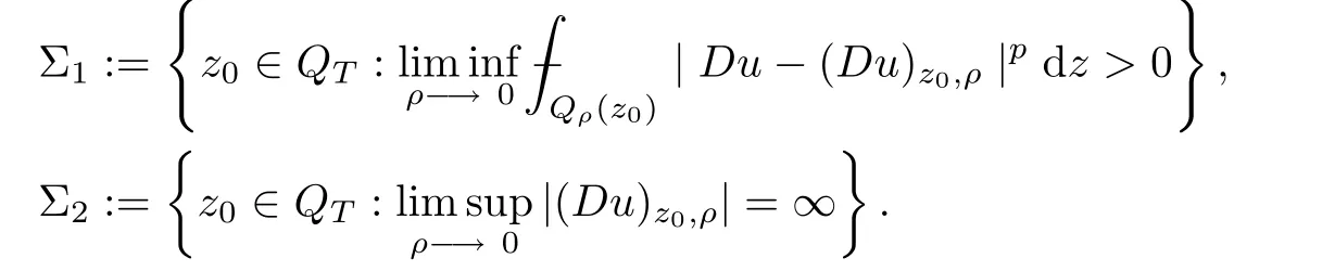
The main technique we have used in the proof of Theorem 1.1 is theA-caloric approximation lemma.Here,Ais a bilinear form on RNn×RNnwith constant coefficients.IfAsatis fies certain growth and ellipticity conditions,then the weak solutionhto(5.6)isA-caloric and has good decay properties.In order to look for such a‘good’function,we shall use theA-caloric approximation lemma(see Lemma 2.7),which enables us to transfer the property of theAcaloric to some‘bad’function(target function).When applying theA-caloric approximation lemma,we need to pay attention to three necessary conditions:
i)the target function is bounded from above on the scale of theL2-norm and theLp-norm;
ii)the target function satis fies a linearized system;
iii)the target function satis fies the smallness condition in the sense of distribution.
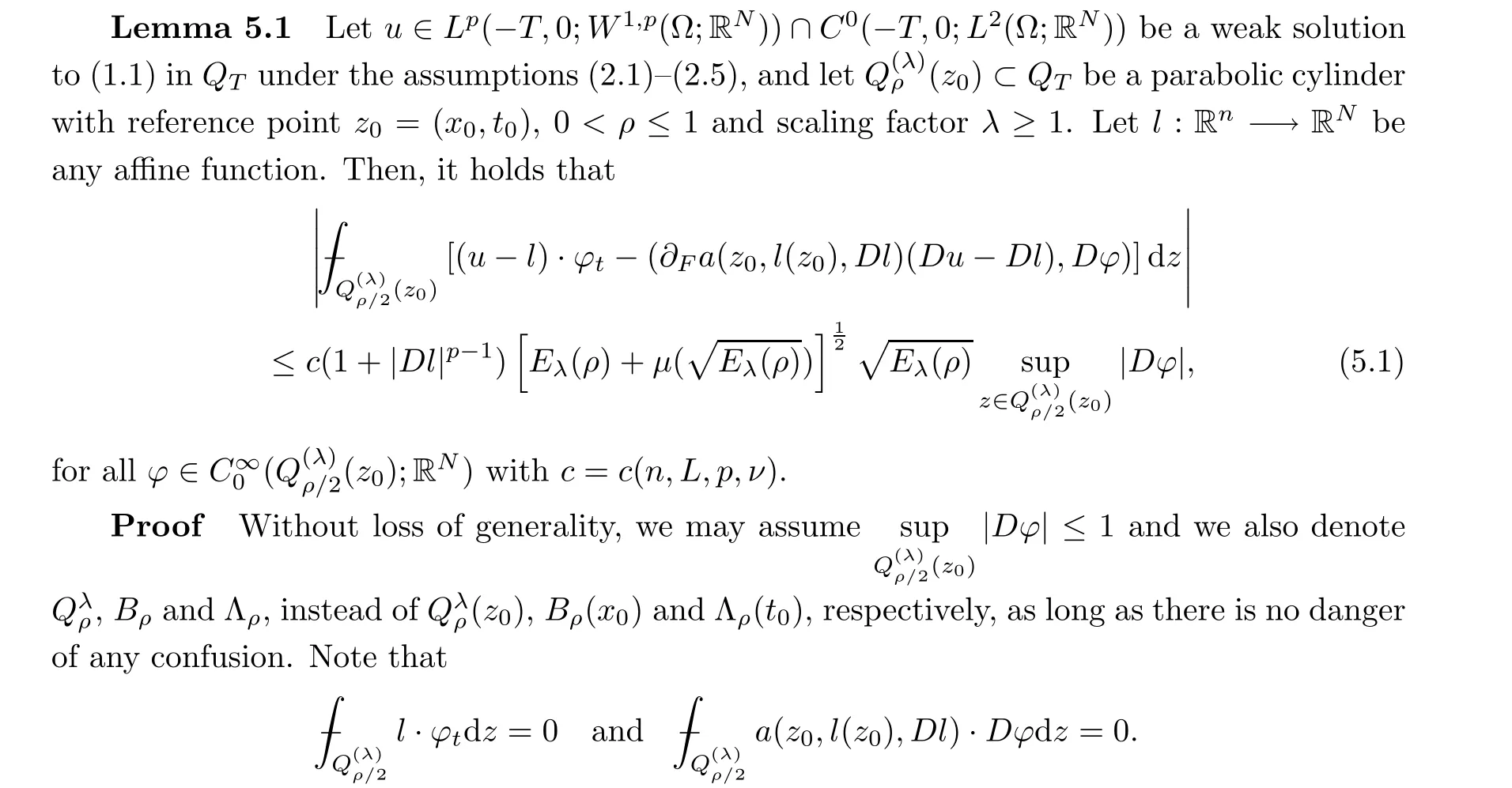
To justify such conditions,we will establish the Caccioppoli inequality and linearize the system(1.1)in Section 3 and Section 5.On the other hand,with the help of a linearization lemma(see Lemma 5.1),we shall show thatw:=u?lρa(bǔ)pproximately solves
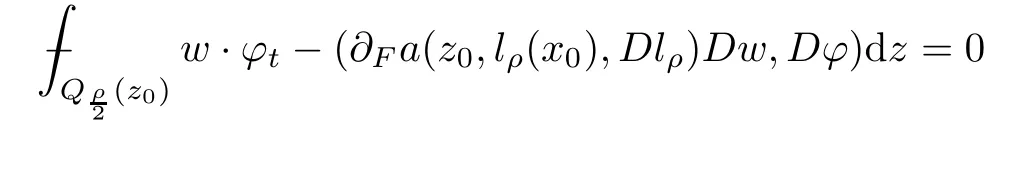
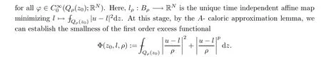
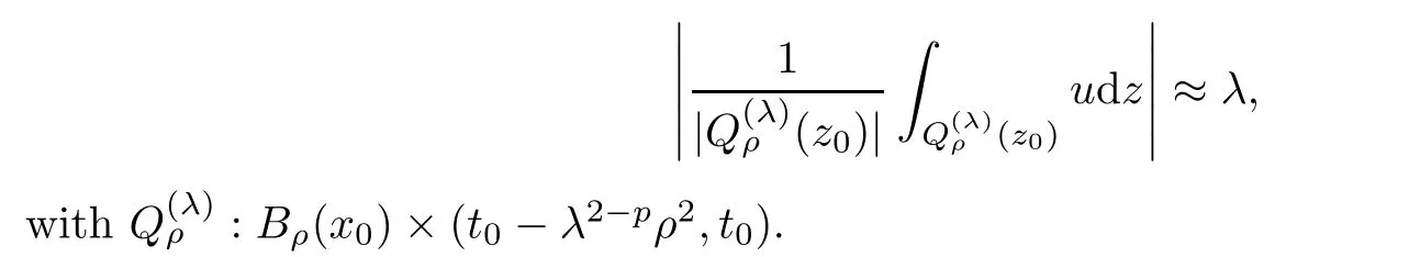
From this,we are able to measure the oscillation inuwith respect to an affine mapping.Moreover,in order to provide a bilinear form that satis fies the growth and ellipticity bounds needed to apply theA-caloric approximation lemma,we may need the integral estimate on intrinsic cylinders,that is,parabolic cylinders stretched according to the size of the solutionuitself.The rough asymptotic is given by
According to Theorem 1.1,we immediately deduce that

whereK:=Σ1∪Σ2and 1K=1 forx∈K;otherwise,1K=0.Then we have the following result:
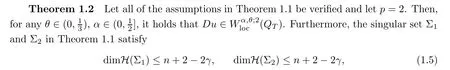
whereγ≤min{α,2θ}.
The rest of this paper is organised as follows:in Section 2,we state some assumptions about the structure functiona(·)and the inhomogeneity termb(·).Moreover,we present some notation,de finition of a weak solution to(1.1),and some useful lemmas which will be used in our proof.Next,in Section 3 and Section 4,we provide some preliminary material which will be quite useful in the proof of main result.The first step of our proof is to establish a Caccioppoli’s type inequality.Subsequently,we establish a Poincartype inequality in Section 4,from which we will be in a position to show the boundness of|Dl|.In Section 5,we first provide a linearizati on strategy for context,then we show a decay estimate of Φλj(?jρ),and finally obtain a Campana to type estimate.This,combined with a standard argument,implies Theorem 1.1.Finally,in Section 6,we derive the fractional time and space differentiability ofDu,from which we estimate the Hausdorff dimension of a singular set of a weak solutionuto(1.1).
2 Preliminaries
2.1 Notation
Lettingx0∈Rn,t0∈R,z0=(x0,t0),we denote
as an open ball in Rn,and let

as a cylinder in Rn+2.LetBρ(x0),Qρ(z0)?QT,andf(x,t)be integrable onBρ(x0)andQρ(z0).Then the average integrals offoverBρ(x0)andQρ(z0)are de fined by
In what follows,we shall repeatedly use the scaled parabolic cylinders of the form
with radiusρ>0,scaling factorλ>0,and
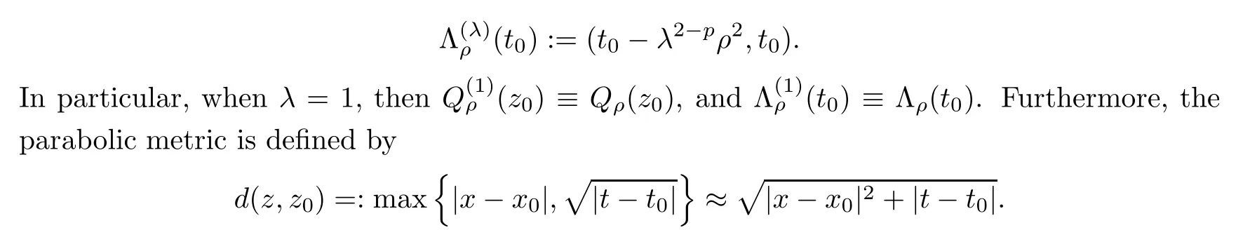
Based on the parabolic metric,the spacesCk;α1,α2(QT)are those of functionsu∈Ck(QT)which areα1-Hlder continuous in the space variables andα2-Hlder continuous in the time variables.More precisely,we say thatu∈Ck;α,α/2(?T;RN)(k≥0 being an integer)if

We say thatu(QT;RN)if and only if,for allA?QT,it holds thatu∈Ck;α,α/2(A;RN).Finally,throughout the paper,we use the notation(·,·)to denote the inner product.Fors∈[0,n+2]andE?Rn+1,we de fine the(parabolic)Hausdorffmeasure as
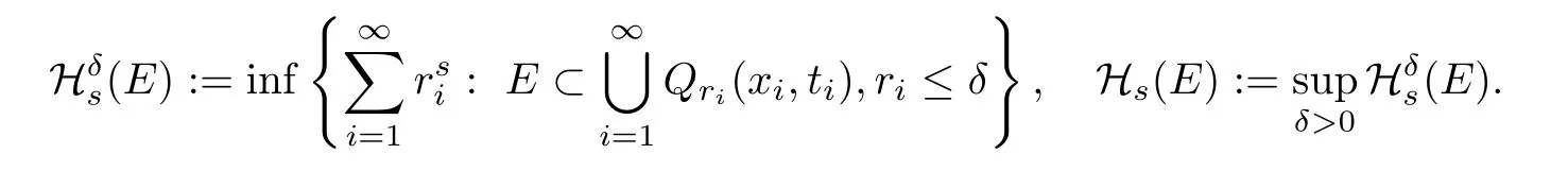
From above,the Hausdorff dimension is usually de fined by

Moreover,in this paper we useDor?to denote the‘gradient’,and we will use the following notations:
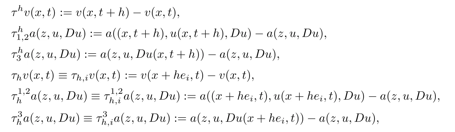
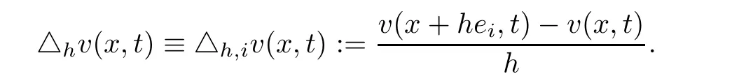
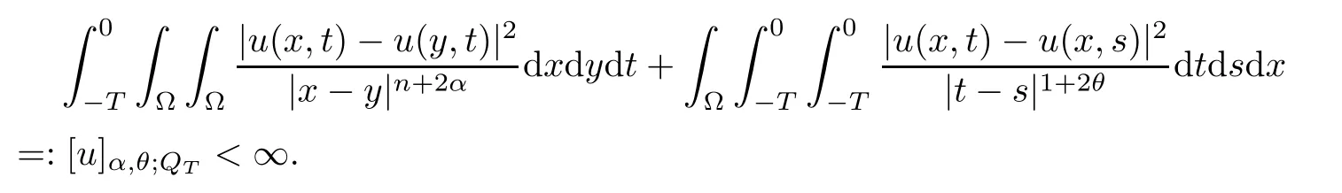
Here,ei=(0,...0,1i?th,0,...,0),i=1,...,n.Finally,let us recall the de finition of parabolic fractional Sobolev space(refer to[36]for details).We say thatu∈L2(QT)belongs to the fractional Sobolev spaceWα,θ;2(QT),α,θ∈(0,1)if
2.2 Assumptions about the structure functions a(·)and b(·)
We impose the condition on the structure functionsa(z,u,F)andb(z,u,F)forp≥2 as follows:
?The growth condition

with(z,u,F)∈QT×RN×RNn,L≥1 being a constant.
?The ellipticity condition

for all(z,u,F)∈QT×RN×RNn,∈RNn,0<ν≤1≤Lbeing a constant.
Moreover,we also need the following two continuity conditions:
?The continuity of lower order term

?The continuity of higher order term

for allz,z0∈QT,u,u0∈RNandF,F0∈RNn.Here,ω,μ:[0,∞)→[0,1]are two bounded,concave,and non-decreasing functions satisfying

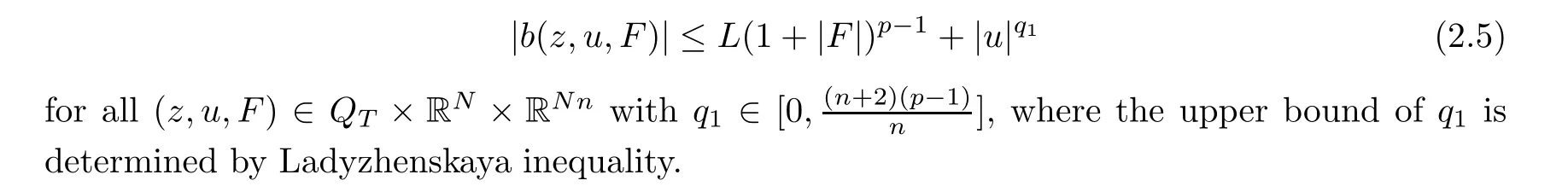
The termb(z,u,F)satis fies a controllable growth condition
2.3 Definition of weak solution
Lettingp≥2,we say thatu∈C0(?T,0;L2(?;RN))∩Lp(?T,0;W1,p(?;RN))is a weak solution to(1.1)if and only if the identity

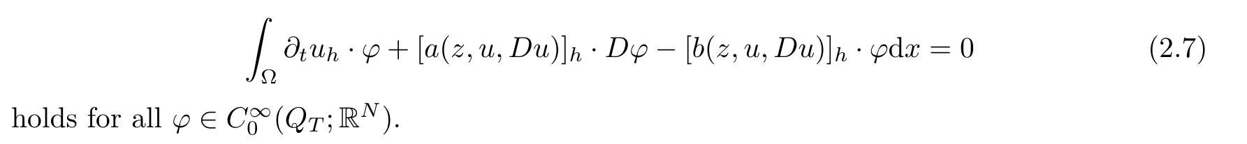
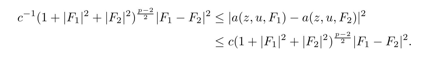
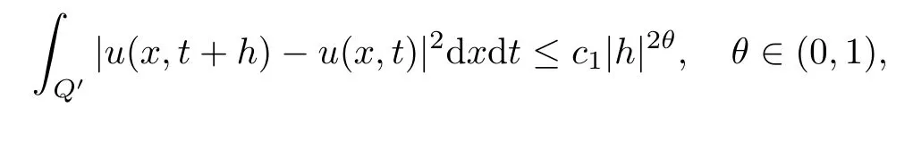
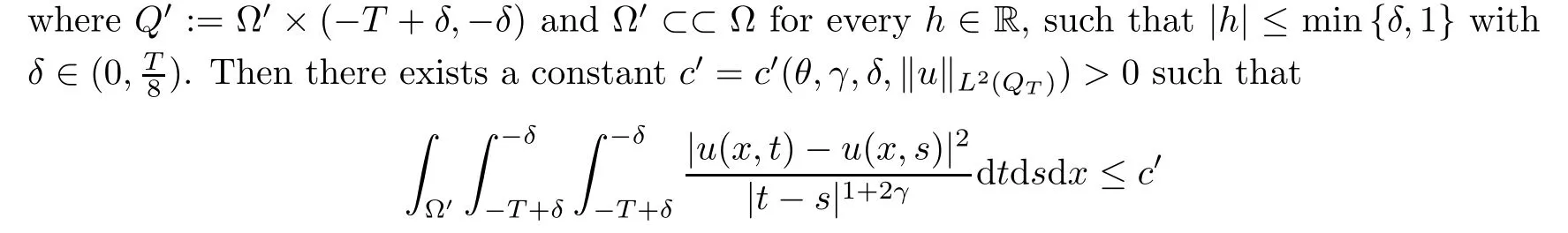
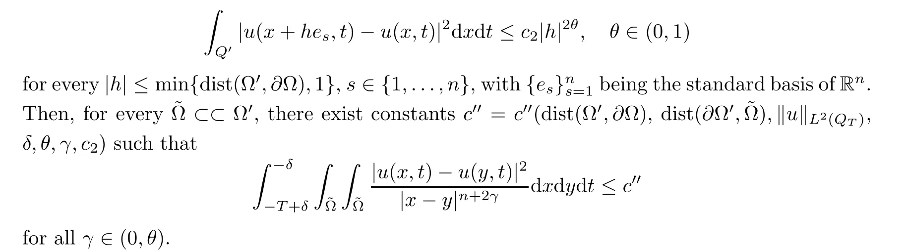
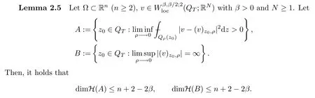
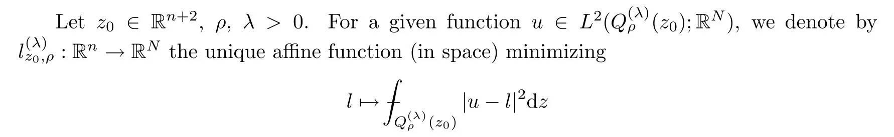
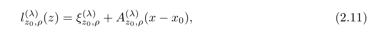
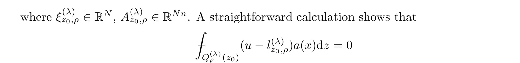
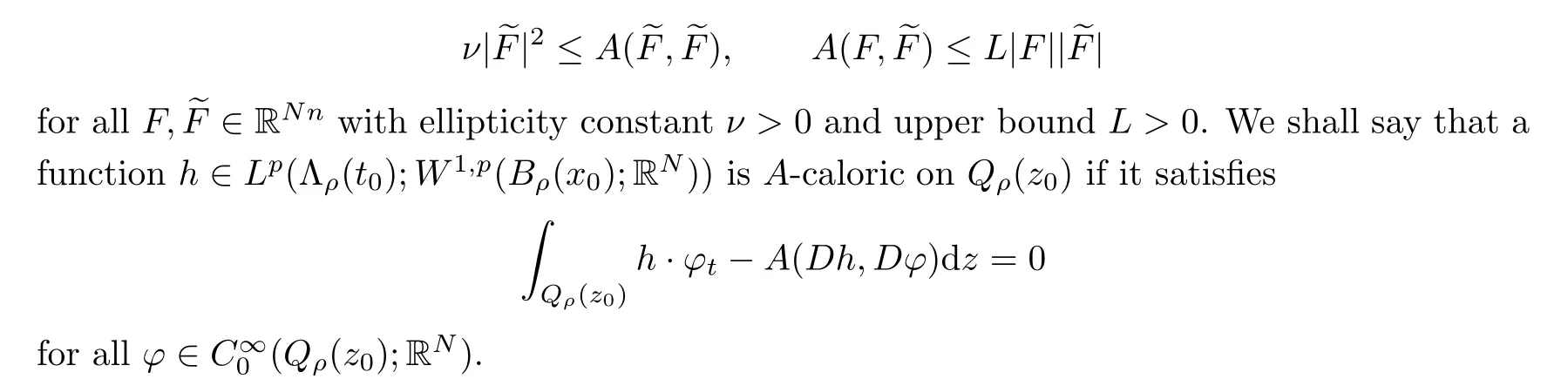
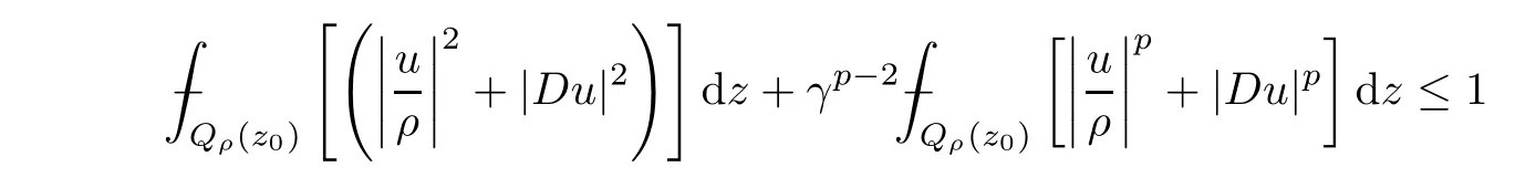
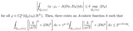
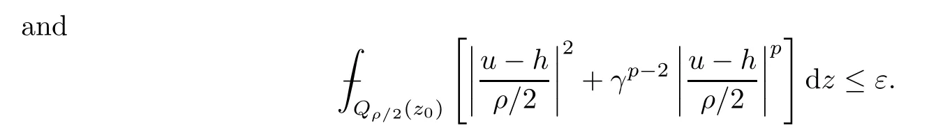
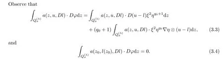
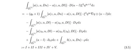
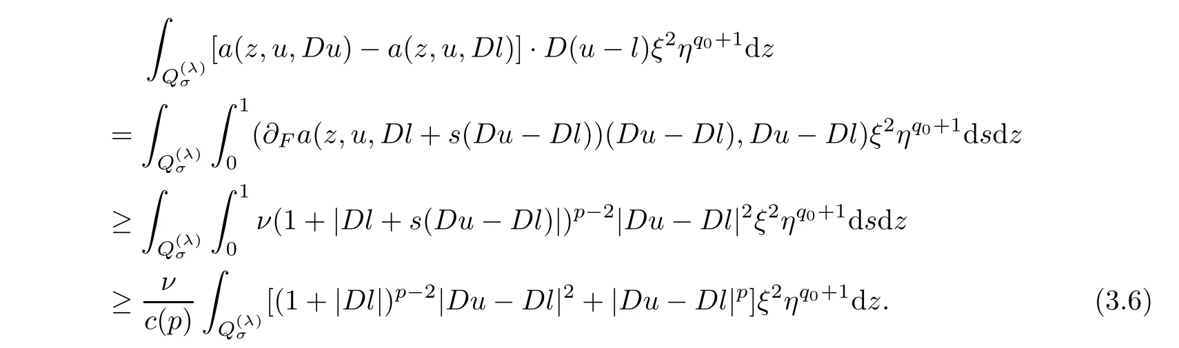
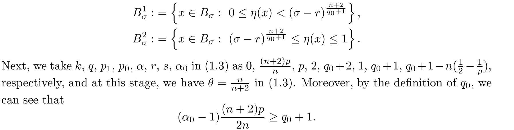
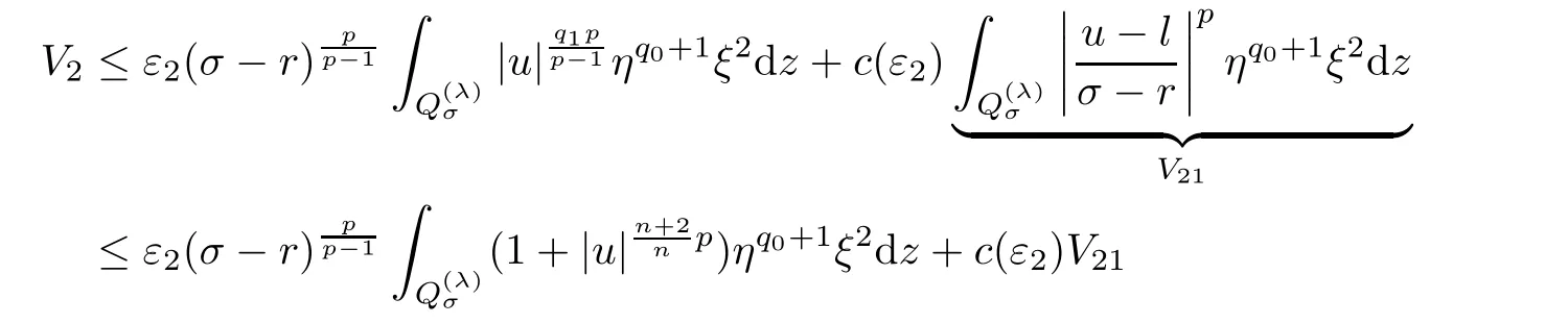
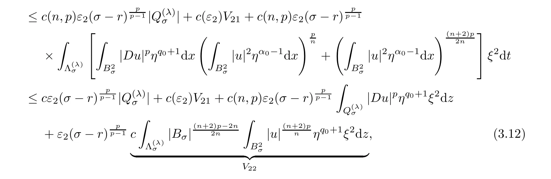
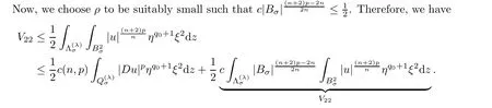
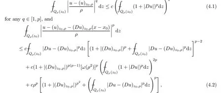
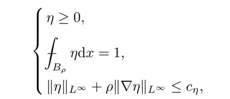
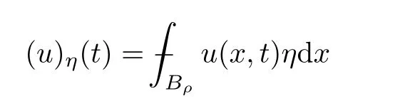
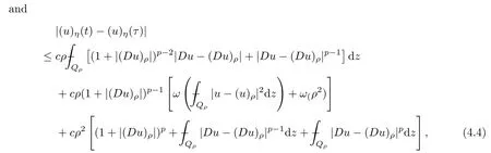
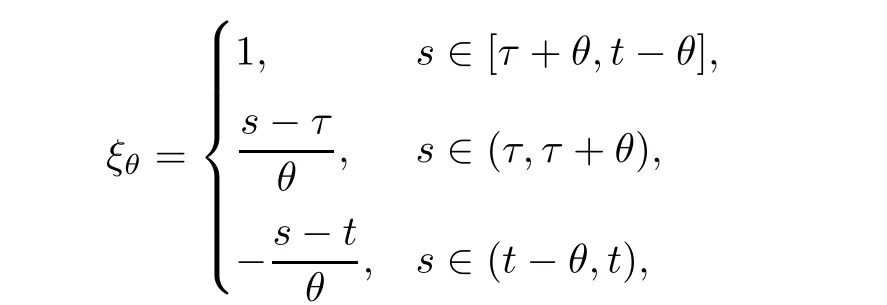
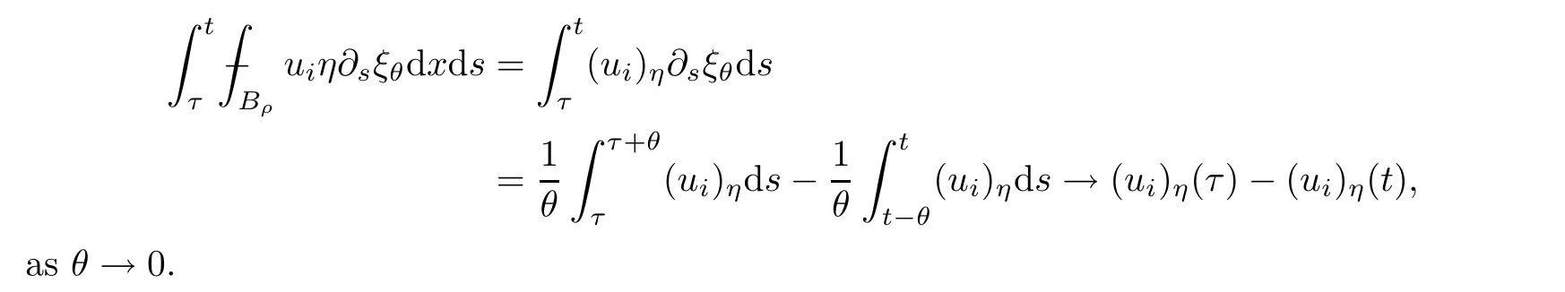
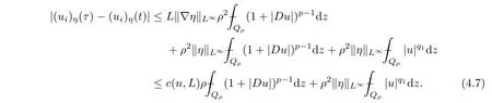
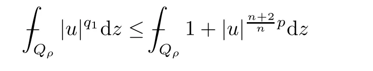
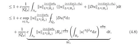
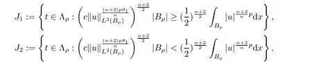
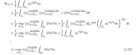
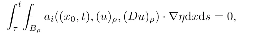
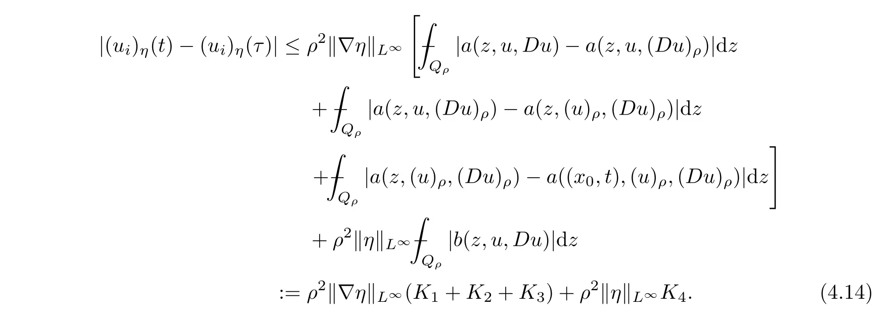
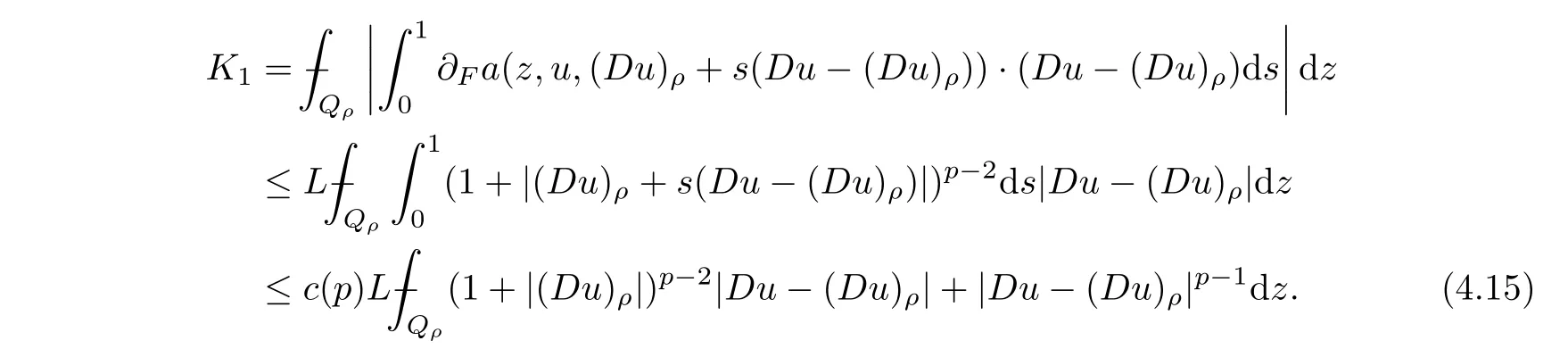
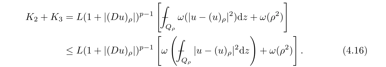
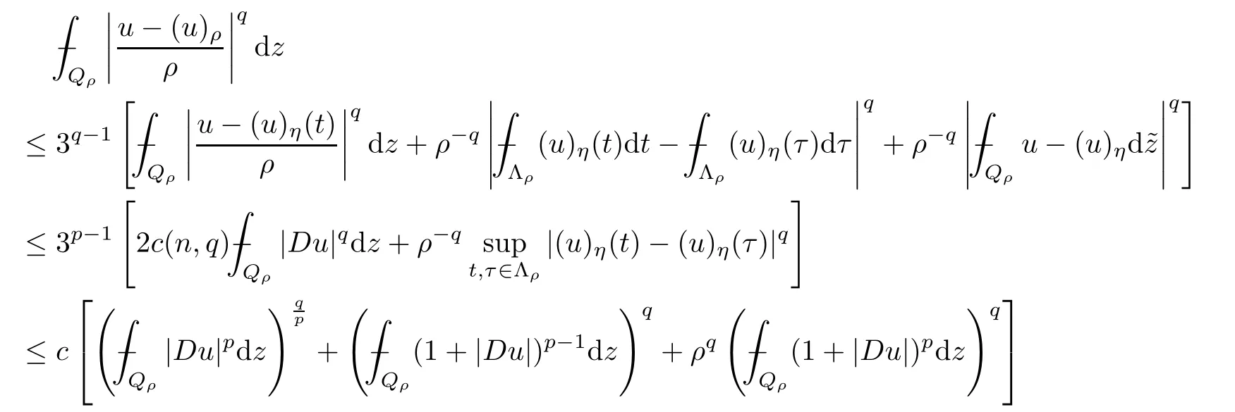
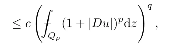
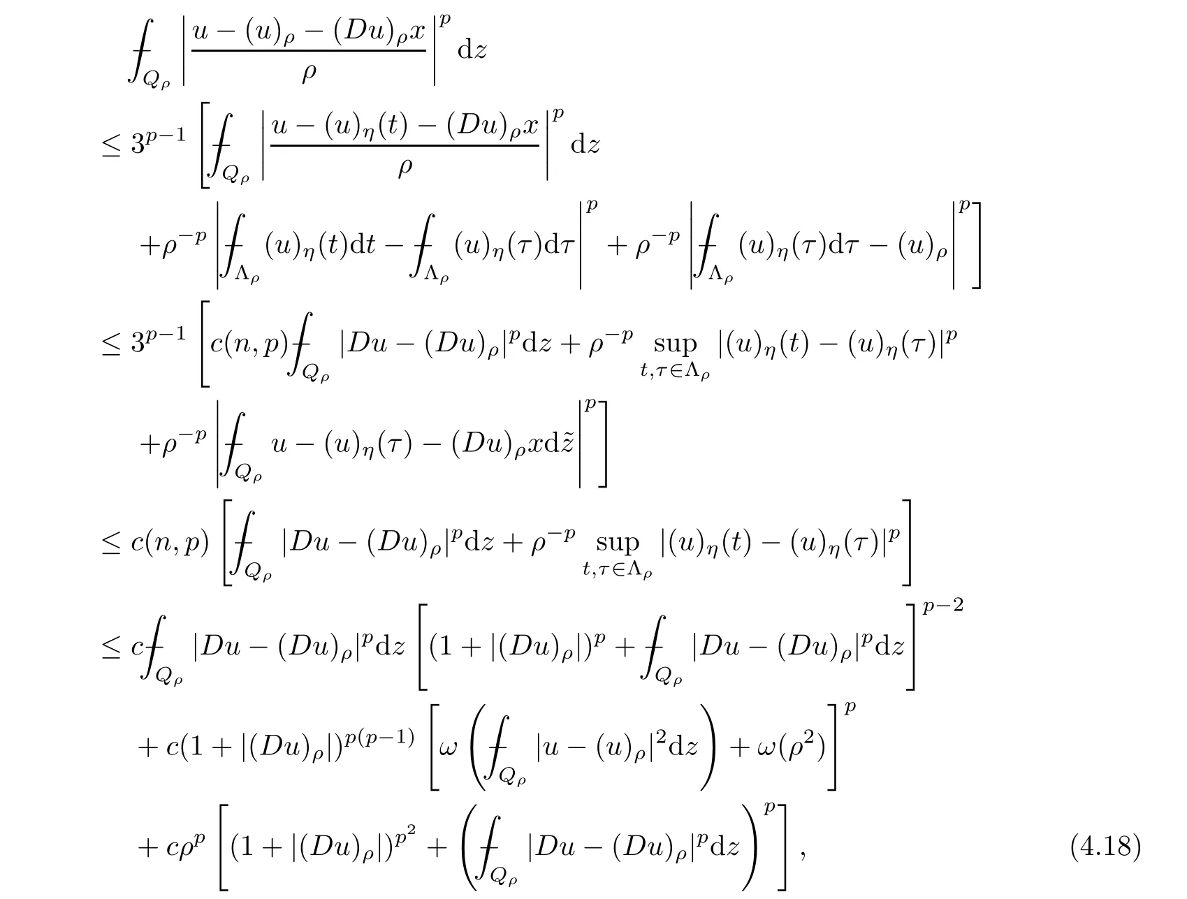
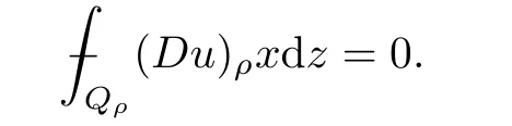
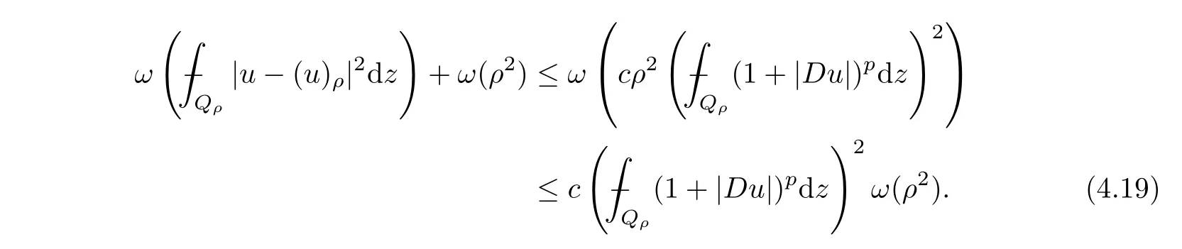
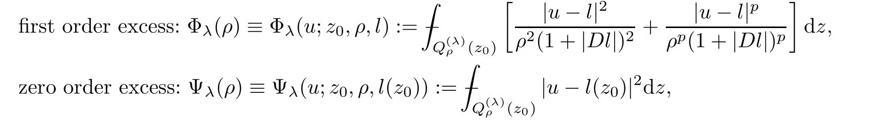
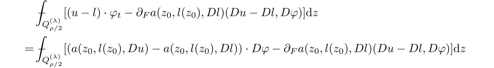
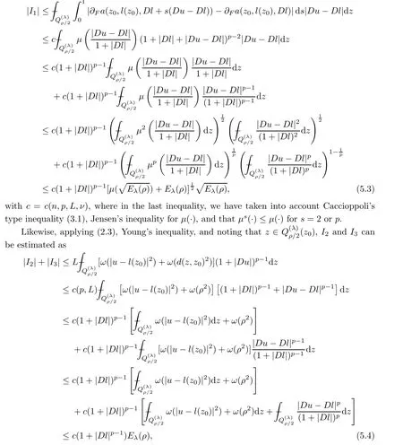
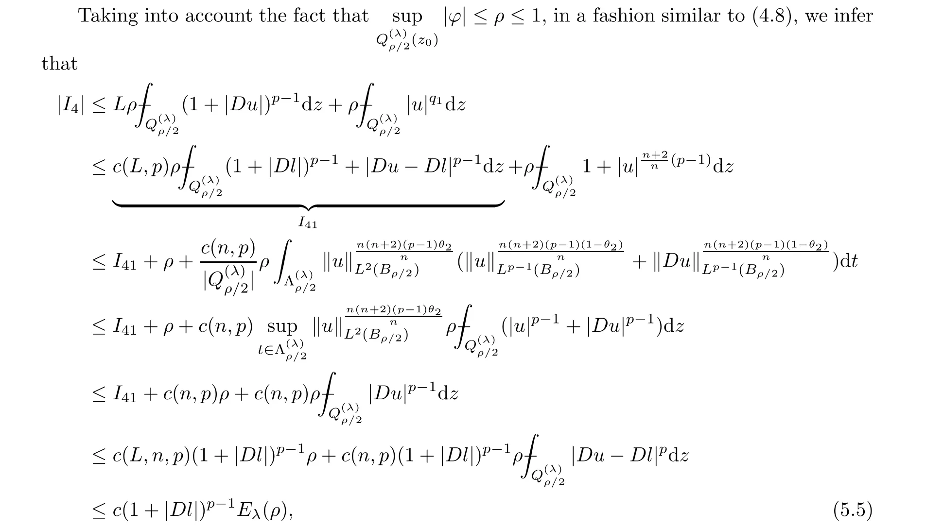
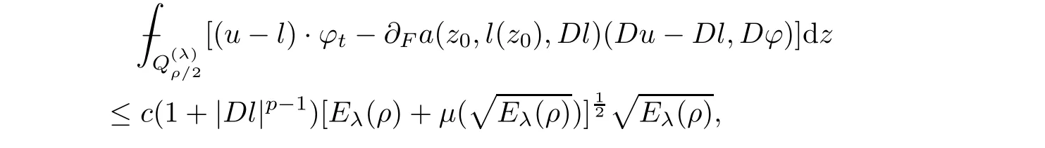
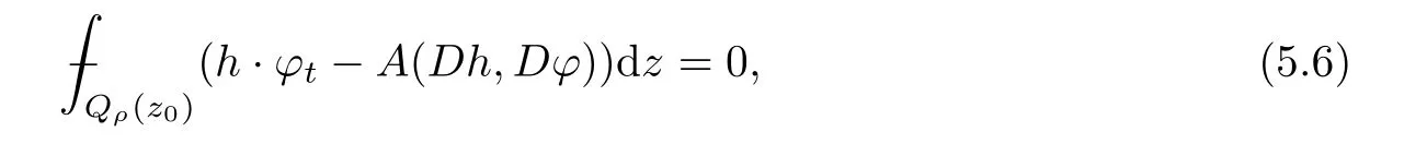
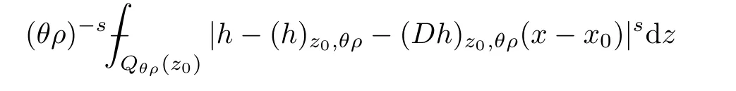
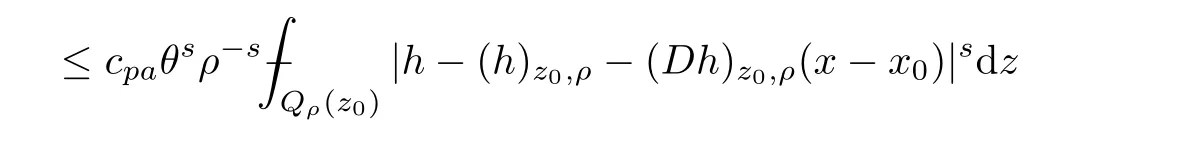
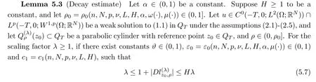
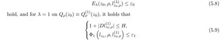
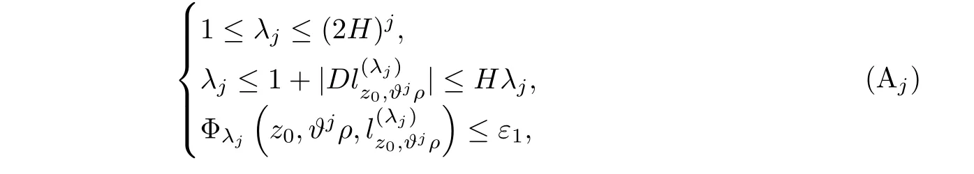
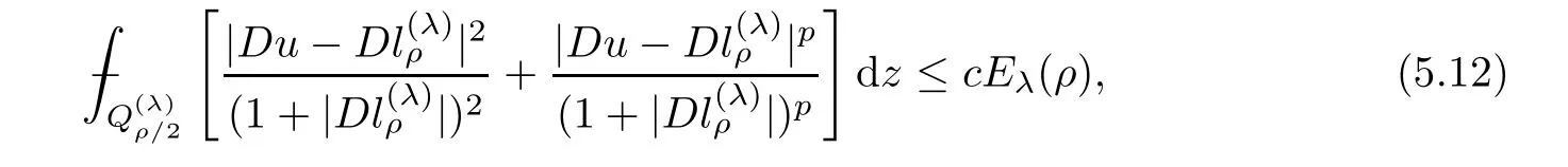
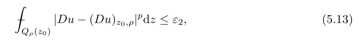
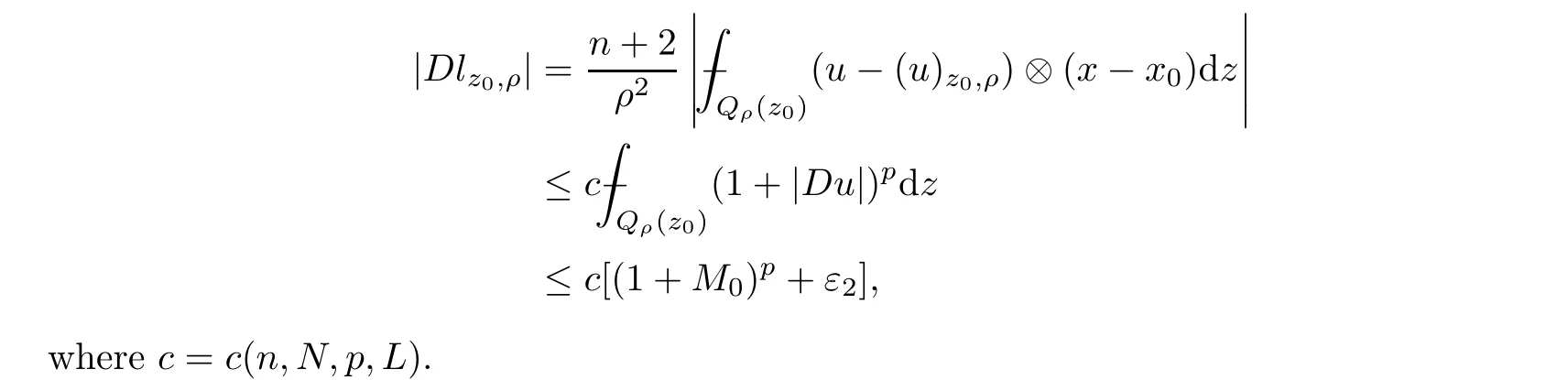
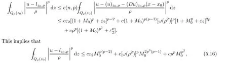
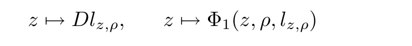
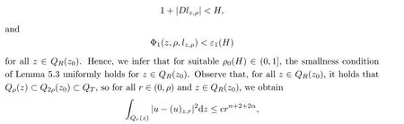
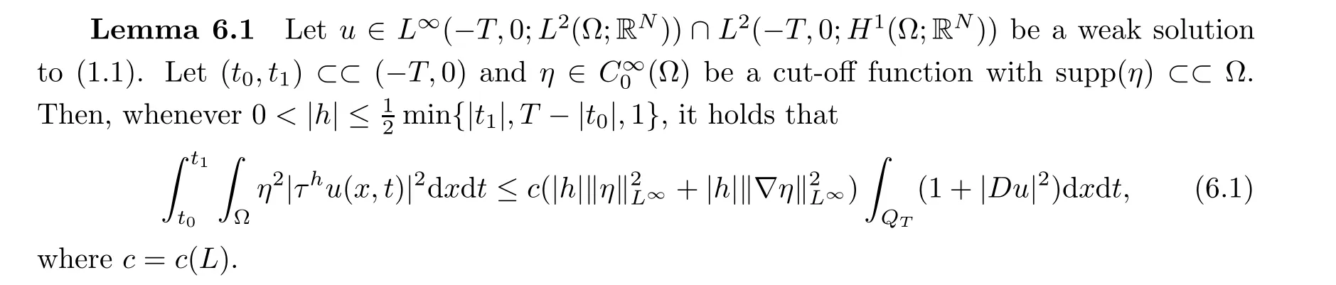
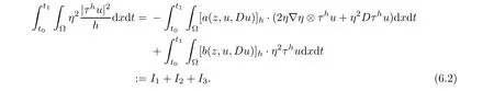
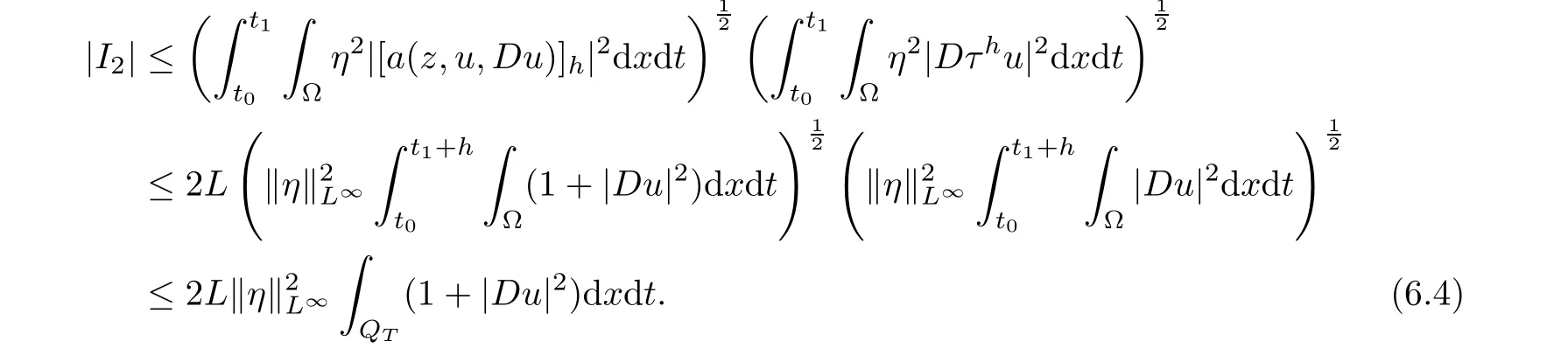
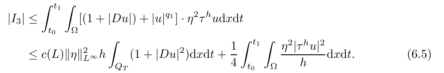
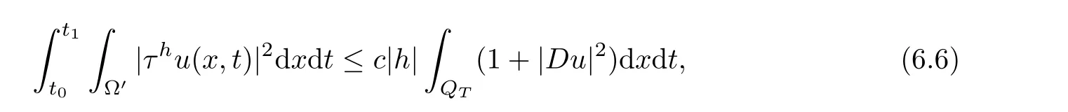
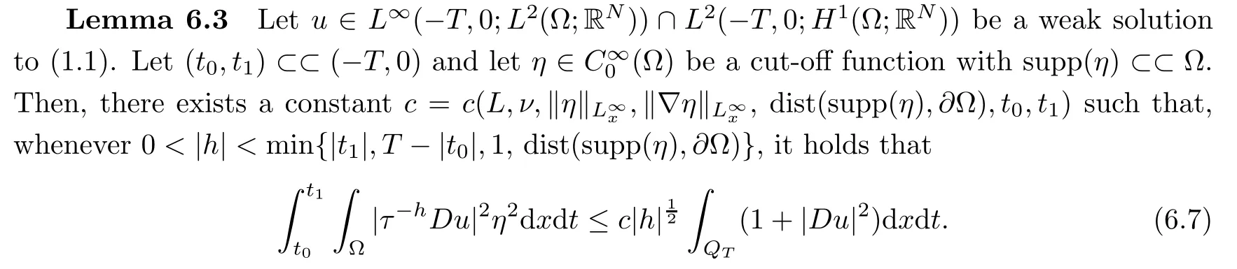
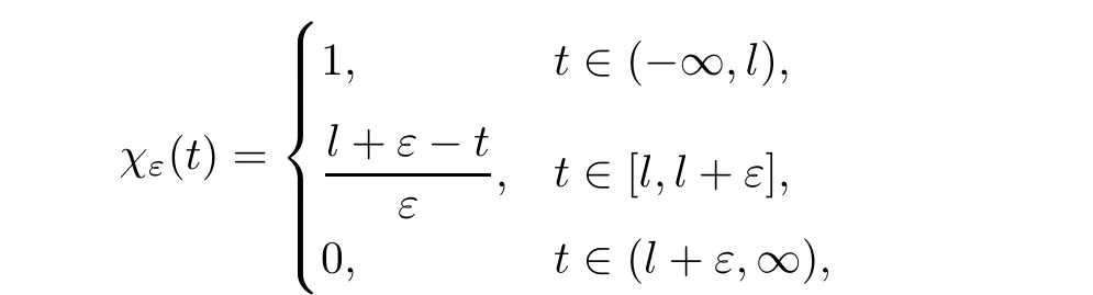
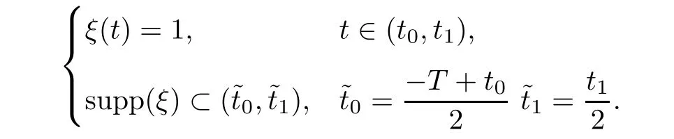
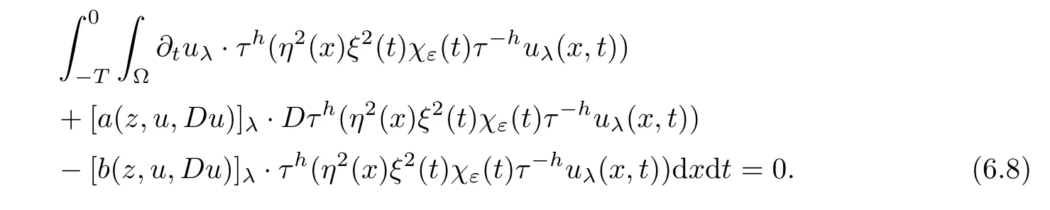
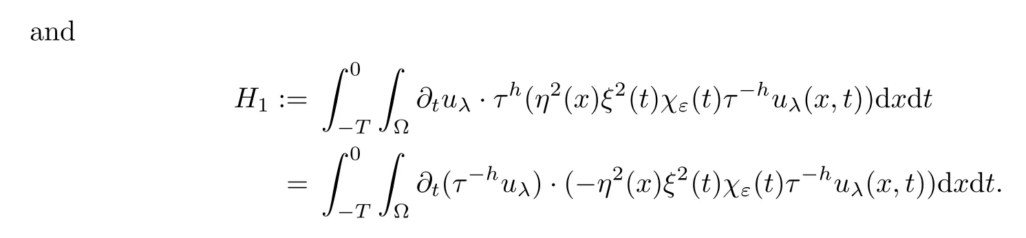
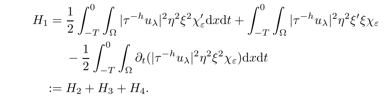
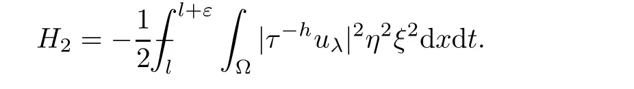
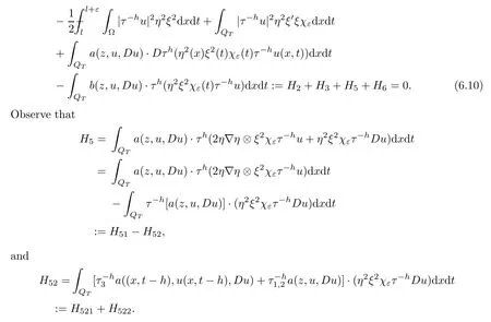
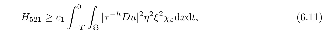
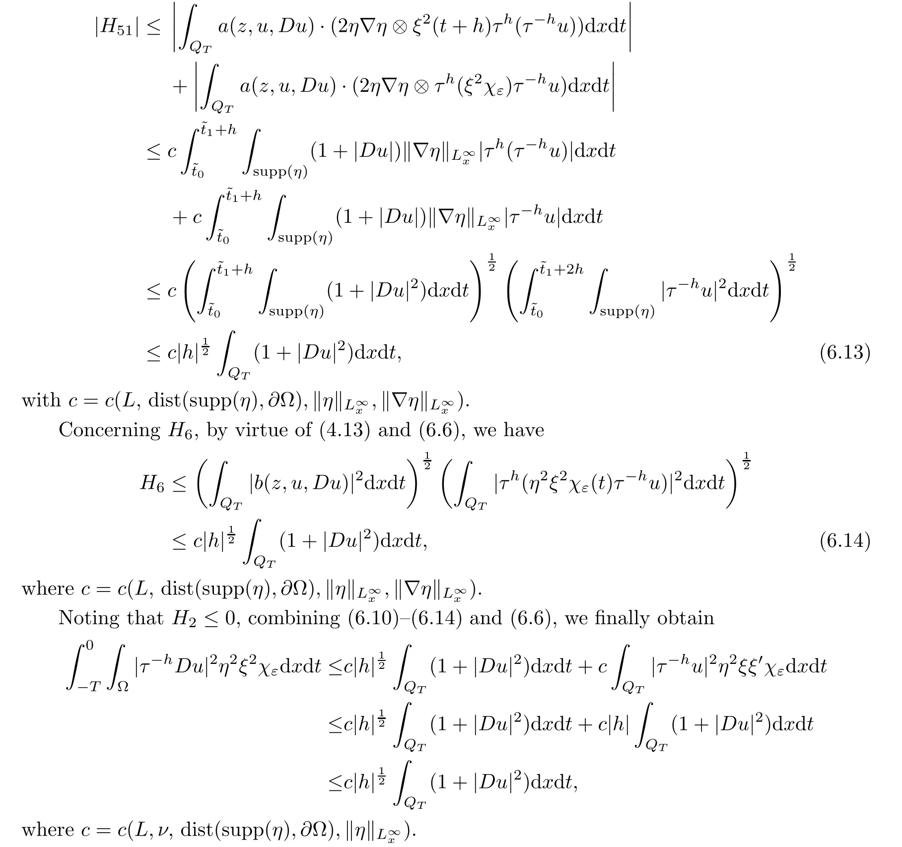
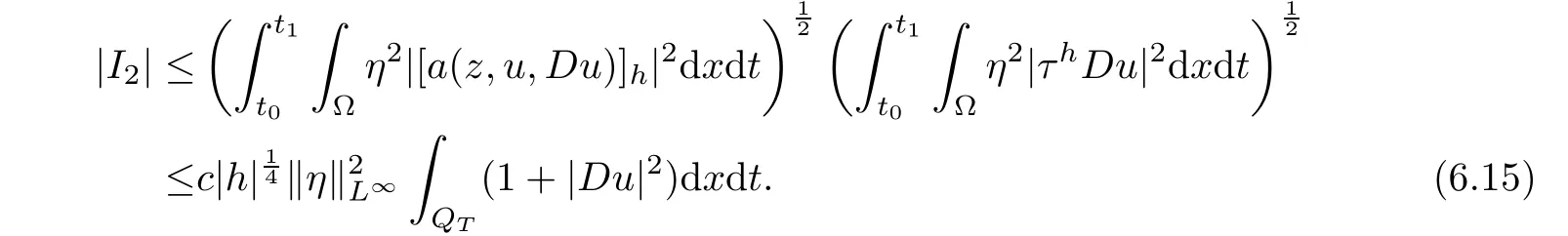
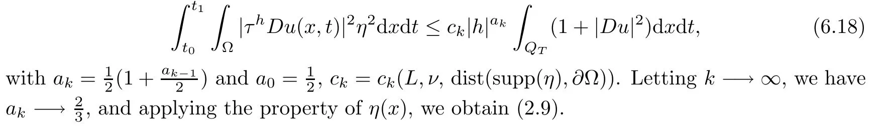
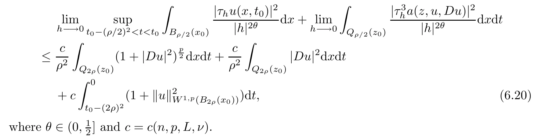
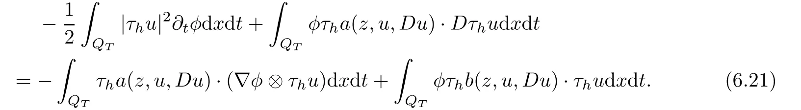
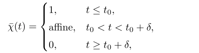
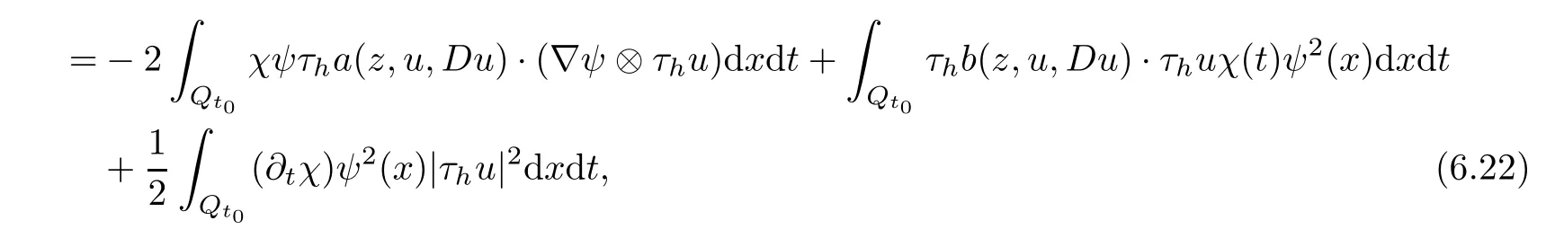
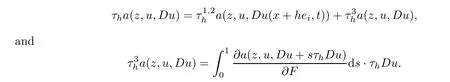
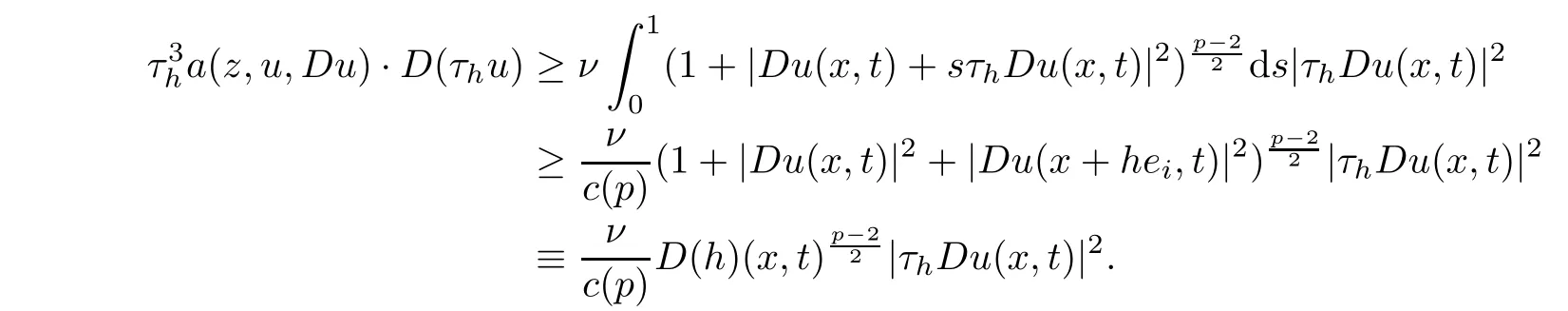
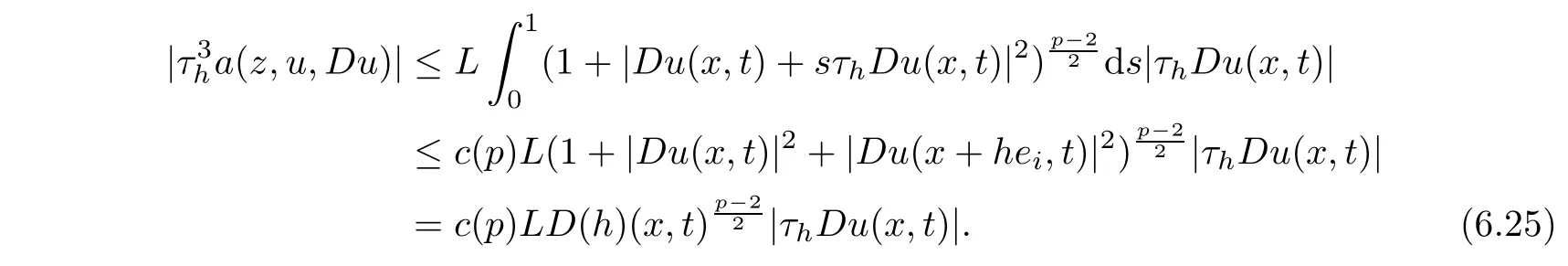
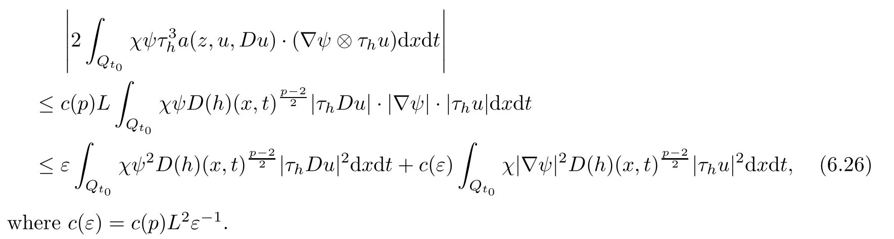
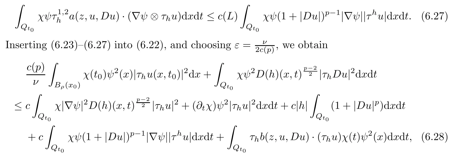
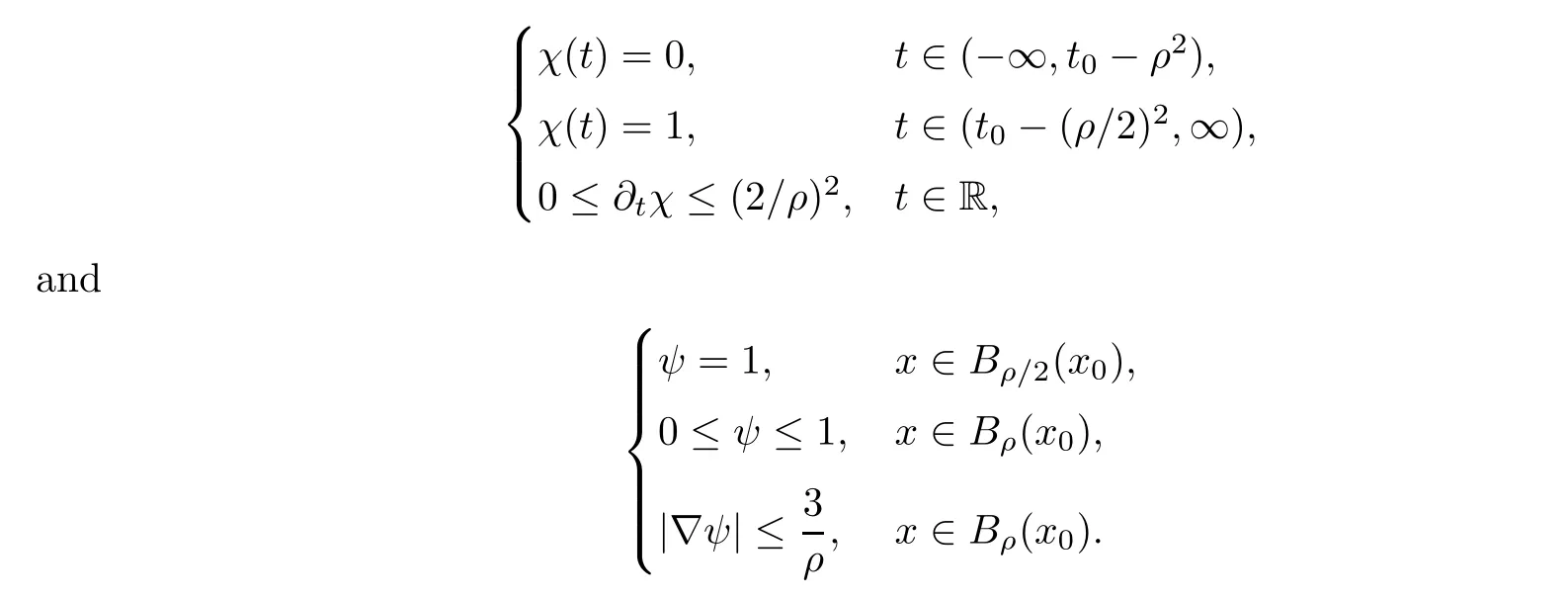
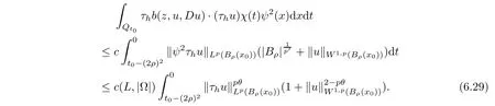
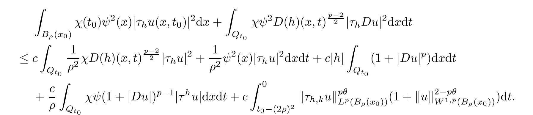
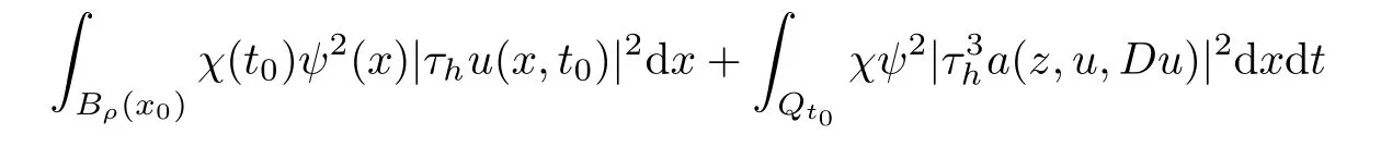
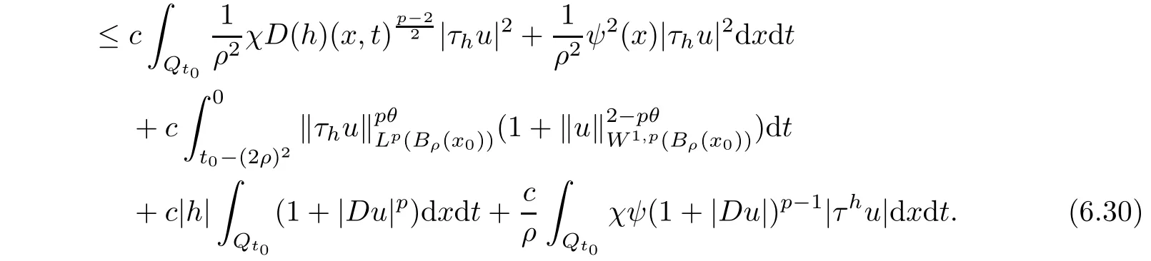
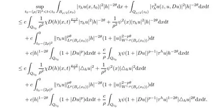
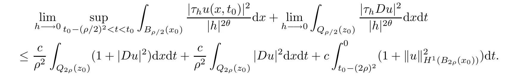
From[19](see also[36]),we recall the definition of the Steklov averages that allow us to restate(2.6)in an equivalent way.Lettingv∈L1(QT)and 0 respectively,for allt∈(?T,0).We note that ifv∈Lr(?T,0;Lq(?))withr,q≥1,thenvh?→vinLr(?T+ε,0;Lq(?))ash?→0 for everyt∈(?T+ε,0)andε∈(0,T),and the same result holds forvˉh. By virtue of the convergence properties of the Steklov averages,we have the following equivalent definition of weak solution to(1.1): Definition 2.1(An equivalent definition of a weak solution)Let 2≤p<∞andu0∈L2(?).Thenu∈L∞(?T,0;L2(?))∩Lp(?T,0;W1,p(?))is called a weak solution to(1.1)if Employing(2.1)and(2.2),we have Lemma 2.2Letting 2≤p<∞,there exists a constantc=c(L,n,p)>0 such that,for anyF1,F2∈RNn,it holds that The following lemma,as an auxiliary tool,will be heavily used in the remainder of the paper(see[14]). Lemma 2.3LetA,B∈Rk,k≥1 andσ>?1.Then there exists a constantc=c(σ),such that As a consequence,from Lemma 2.3 and(2.2),it follows that the monotonicity ofa(z,u,·)is wherec=c(n,p,ν). In the next proposition we recall the parabolic version of the well known relation between Nikolski spaces and Fractional Sobolev spaces(see[42]). Proposition 2.4Lettingu∈L2(QT;RN),suppose that for allγ∈(0,θ).Furthermore,suppose that From Proposition 2.4,we can see that in order to prove the fractional differentiability ofDuin Theorem 1.2,it is only needed to prove On the other hand,for estimating the Hausdorff dimension of singular set ofude fined in Theorem 1.1,we shall use the following arguments(see[23,38]): amongst all affine functionl(z)=l(x)independent oft.We note that such a unique minimizing affine function exists and takes the form for anya(x)=ξ+A(x?x0)withξ∈RN,A∈RNn.This implies,in particular,that Furthermore,we need the following argument,which can be proven analogously to[49]:for anyξ∈RnandA∈RNn,it holds that A strongly elliptic bilinear formAon RNnmeans that In order to obtain the decay estimate(5.11),we introduce the followingA-caloric approximation lemma(see[29]). Lemma 2.7There exists a positive functionδ0=δ0(n,p,ν,L,ε)∈(0,1]with the property that,for eachγ∈(0,1],and each bilinear formAin RNnwith ellipticity constantνand upper boundL,εis a positive number wheneveru∈Lp(Λρ(t0);W1,p(Bρ(x0);RN))satisfying is approximatelyA-caloric,in the sense that for eachδ∈(0,δ0]it holds that In this section,we propose to derive a Caccioppoli type inequality under the conditions(2.1)–(2.3)and(2.5).Such a result provides a bridge between theA-caloric approximate lemma and Lemma 5.1. Lemma 3.1(Caccioppoli type inequality)Letu∈C0(?T,0;L2(?;RN))∩Lp(?T,0;W1,p(?;RN))be a weak solution to(1.1)under the assumptions(2.1)–(2.3)and(2.5),and letbe a scaled parabolic cylinder with reference pointz0=(x0,t0)and 0<ρ≤1 being suitably small,with scaling factorλ≥1 and affine functionl:Rn→RNsuch thatλ≤1+|Dl|.Then it holds that Thus,inserting(3.3)–(3.4)into(3.2)and noting thatl(z)=l(x),we arrive at Firstly,we focus our attention on estimating the term on the left side of(3.5).Appealing to(2.2)and Lemma 2.3,we infer that Now,we turn to estimating the termsI?Vin(3.5).For the termI,we first note that,from(2.1),it holds that whereε∈(0,1)will be specified later,and in the previous inequality,we have taken into account that|Du|≤|Dl|+|Du?Dl|. Next,using(2.3),we deduce that For termIV,note thatλ≤1+|Dl|,so we have Finally,we estimate termV.From(2.5),we have By Young’s inequality,it is clear that withε1∈(0,1)to bespeci fied later. For termV2,first we divideBσinto two parts:and Therefore,by the weighted Sobolev interpolation inequality(1.3)and Hlder’s inequality,we are in a position to obtain whereε2∈(0,1)will be specified in later. This implies that As a consequence,from(3.12)–(3.13),it follows that Inserting(3.6)–(3.11)and(3.14)into(3.5),we conclude that and lettingδ1→0,we have(3.1). In this section,we aim to establish a Poincartype inequality of a weak solution to(1.1)under the assumptions(2.1),(2.3)and(2.5).We note that such an inequality plays a key role in this paper,especially in Section 5,where we will show that for everyz0∈QT(Σ1∪Σ2)and suitable 0≤ρ0≤1,the assumption of Lemma 5.3 is valid. Lemma 4.1(Poincartype inequality)Letu∈Lp(?T,0;W1,p(?;RN))∩C0(?T,0;L2(?;RN))be a weak solution of(1.1)inQTunder the assumptions(2.1),(2.3)and(2.5),withQρ(z0)?QTbeing a parabolic cylinder with referencez0=(x0,t0)and 0<ρ≤1.Then,it holds that wherec=c(n,N,p,L). ProofFor simplicity,we may also omit the reference pointz0ofQρ(z0),Bρ(z0)and Λρ(z0),using insteadQρ,Bρa(bǔ)nd Λρ,respectively,as long as there is no danger of any confusion.Letbe a nonnegative weight function satisfying wherecη=cη(n),and de fine as a weighted mean ofu(x,t)onBρfor a.e.t∈(?T,0).To begin with,we shall show the following argument for a.e.t,τ∈Λρ: wherec=c(n,N,p,L). Now,we concentrate our attention on the proof of(4.3)–(4.4).Without loss of generality,we may assume thatt>τ,and letξθ(s)∈((τ,t))be a cut-offfunction,de fined by withθ∈(0,(t?τ)/2).We now choose?θ:Rn+2→RNto be a test function in the weak formulation(2.6)with(?θ)i=ηξθand(?θ)j=0 forj/=iandi,j∈{1,...,N},which implies that Taking intoaccount the Steklov arguments and the definition of(u)η(t),we first deduce that Next,lettingθ→0 in the right side of(4.5),we arrive at By virtue of(2.5),(4.6),and noting thatt,τ∈Λρ,we infer that Now we focus our attention on estimating the rightmost term in(4.7).Employing an interpolation inequality(G-N-S inequality),it holds that where in the last inequality we have taken into account that It is clear that the termW1can be split as where Λρ=J1∪J2,and Thus,we are in a position to obtain and,by iteratively estimating,we have Plugging(4.10)–(4.12)into(4.8),we conclude that Now,combining(4.13)and(4.7),and summing up overi=1,...,N,we have(4.3).Hence,it remains to prove(4.4). Observing that and making use of(4.6),we infer that Applying(2.1)and Lemma 2.3,for the termK1we have In addition,making use of(2.3)and Jensen’s inequality,the termsK2andK3can be estimated as For the termK4,in view of(4.6)–(4.7)and(4.13),we have Inserting(4.15)–(4.17)into(4.14),and summing up overi=1,...,N,we get(4.4). Now,we turn to proving(4.1)–(4.2).First,appealing to(4.3),Poincar’s inequality with a weighed function,and Hlder’s inequality,we infer that where=(x,τ)andc=c(n,N,p,L).Thus,we have(4.1). withc=c(n,N,p,L),where in the second inequality,we have used Poincar’s inequality for a.e.t∈Λρa(bǔ)nd the fact that Taking into account the concavity ofω(·),and(4.1)forq=2,implies that Thus,combining(4.18)and(4.19),we are in a position to obtain whence we get(4.2). According to Lemma 3.1,we now de fine some excess functionals.For reference pointz0=(x0,t0)∈QT,u∈Lp(?T,0;W1,p(?;RN)),affine functionl:Rn→RN,andl(z)=l(x),in what follows we denote and hybrid excess functional The following lemma is a prerequisite for applying theA-caloric approximation technique: Then,from weak formulation(2.6),we deduce that Now we start to estimateI1–I4.For the termI1,applying(2.4),as well as the Hlder and Young inequalities,we have wherec=c(n,p,ν,L). wherec=c(n,p,L,ν)andθ2∈(0,1)is the same as withθ1in(4.9). Plugging(5.3)–(5.5)into(5.2),we have wherec=c(n,p,ν,L).By a general scaling argument,we have(5.1). The aim of this section is to provide a decay estimate of Φλj(z0,?jρ,lj),withλj,?,ljto be speci fied in later,from which we can obtain a Campanato type estimate of a weak solutionuto(1.1),then derive the regularity ofuby a standard argument from Campanato space.First,we introduce a standard estimate for a weak solution to linear parabolic systems with constant coefficients(see[15]Lemma 5.1),which is necessary in the proof of the decay estimate of‖u?(u)z0,r‖L2(Qr(z0)). Lemma 5.2Leth∈L2(Λρ(t0);W1,2(Bρ(x0);RN))be a weak solution inQρ(z0)of the following linear parabolic system with constant coefficients: for any∈RNn.Then,his smooth inQρ(z0),and for alls≥1,θ∈(0,1],it holds that for a constantcpa=cpa(n,N,L/ν)≥1. TheA-caloric approximation lemma(Lemma 2.7)allows one to translate these decay estimates onhinto a certain excess functional.This eventually allows one to derive the partial regularity ofu.Based on Lemmas 5.1–5.2,we have the following result: and the smallness condition and for anyr∈(0,ρ],it holds that wherec=c(n,N,p,ν,L,H,α). ProofIn virtue of(3.1)we can see that wherec=c(n,p,ν,L),and.At this stage,by Lemma 5.1,Lemma 5.2 and an iteration argument,one can prove(5.7)–(5.11);the process is similar to the proof of main theorem in[11],here we just skip it. According to Lemma 4.1 and Lemma 5.3,we now are able to prove Theorem 1.1. Proof of Theorem 1.1Letz0∈QT(Σ1∪Σ2).Then by the de finitions of Σ1and Σ2,there exist some constantsε2∈(0,1],M0≥1 such that Now,in virtue of(2.12),(5.13),(5.14)and(4.1),we are in a position to obtain Sinceε2≤1≤M0,the previous inequality implies that Furthermore,by the minimality oflz0,ρ,(4.2)and(5.13)–(5.14),we can see that withc=c(n,N,p,L). Appealing to(5.15)–(5.16),for suitably smallε2∈(0,1),we can deduce the existence ofH≥1 and 0<ρ≤ρ0(H)such thatQ2ρ(z0)?QT,and at this stage,we further obtain that Note that the mappings are continuous.Thus,there existssuch that withc=c(n,N,p,ν,L,H,α).By the Campanato space argument(see[18]),we haveu∈C0;α,α/2in a neighborhood of any pointz0∈QT(Σ1∪Σ2),and we further obtain|Σ1∪Σ2|=0,which means|Q0|=|QT|. In this section,with Theorem 1.1 in hand,we proceed to prove Theorem 1.2.This will be achieved by combining the fractional time and fractional space differentiability of the gradient of weak solutionuto(1.1). In this subsection,we aim to prove the fractional time differentiability ofDuforp=2.First,we estimate theL2-norm ofτhu. ProofFirst,we restrict ourselves to the caseh>0.Choosingη2τhuas a test function in the Steklov averages formulation of(2.7),and integrating with respect tot∈(t0,t1),we deduce Taking into account(2.1),(2.3)and Young’s inequality,it holds that For the termI2,from Hlder’s inequality,it follows that Similarly,forp=2,by applying(4.8)–(4.13),the termI3can be estimated as Finally,we note that the estimation in the other one is the same usinguˉhinstead ofuh.Now,inserting(6.3)–(6.5)into(6.2),we obtain wherec=c(L).Thus,we have(6.1). From Lemma 6.1,we have the following direct result: Remark 6.2Letu∈L∞(?T,0;L2(?;RN))∩L2(?T,0;H1(?;RN))be a weak solution to(1.1).Let(t0,t1)??(?T,0)and ?′???.Then,whenever,it holds that wherec=c(L,dist(?′,??)). Based on Lemma 6.1,we now propose to estimate the time derivative ofDu,which will be regarded as the starting point of an iteration process. ProofWe chooseχε:R[0,1]to be a continuous affine function satisfying approximating the characteristic function of(?∞,l)withl∈(?T,0).Letξ(t)andη(x)be cut-offfunctions in the time and space variables,respectively,such that We takeφ(x,t)=τh(η2(x)ξ2(t)χε(t)τ?huλ(x,t))as a test function in(2.7),and integrating in time respect to(?T,0)yields that We first note that This,combined with(6.9),implies that Recalling the de finition ofχε,we find that Moreover,note thatH4=0.Then,by passing to the limit forλ?→0 in(6.8),we obtain By the aid of(2.8),it holds that wherec1depends onν.Furthermore,applying(2.3),(1.4)and Young’s inequality,it holds that For the termH51,making use of(6.6),we obtain Applying the properties ofξ(t)andη(x),and lettingε?→0 andl?→0,we have(6.7). According to(6.7),we can re-estimate the termI2in(6.4)as follows: From(6.15),and noting that|h|<1,we can rewrite(6.6)as wherec2=c2(L,ν,dist(supp(η),??)). Similarly,in the proof of Lemma 6.3,we can use(6.16)instead of(6.6)to arrive at As with the estimation of(6.15)–(6.17),by an iteration argument,we finally obtain In this subsection,we propose to deduce the fractional space differentiability of the gradient of the weak solutionuto(1.1).To begin with,we discuss the general case forp≥2. Lemma 6.4Let ??Rn(n=2,3)be a bounded domain.Letu∈L∞(?T,0;L2(?;RN))∩Lp(?T,0;W1,p(?;RN))(p≥2)be a weak solution to(1.1).Then,we have and for anyQ2ρ(z0)?QT,it holds that ProofFirst,replace the test function?in(2.6)byτ?h?with Then we infer that By approximation,we choose?≡φτhuin the previous equation with.Thus,we are in a position to obtain that Now,let us chooseφ(x,t)=(t)χ(t)ψ2(x)withχ∈W1,∞((?T,0)),χ(?T)=0,?tχ≥0 and 0≤χ≤1,,0≤ψ≤1 andχˉ:(?T,0)?→R being a Lipschitz continuous function,de fined by with?T whereQt0:=Bρ(x0)×(?T,t0). We observe that Then,applying(2.2)and Lemma 2.3,we can find that Here we have used abbreviated notation Thus,we conclude that Moreover,from(2.3)and(1.4),it follows that Using(2.1),we further obtain that Therefore,applying(6.25)and Young’s inequality,we have Furthermore,by virtue of(2.3),it holds that wherec=c(n,L,p,ν). LetQρ(z0)?QTwithρsuitably small such that 2ρ Note that,for anyθ∈(0],the right-most term of(6.28)can be estimated as Employing(6.28)and(6.29),we finally obtain By Lemma 2.2,the previous inequality implies that Dividing both sides in(6.30)by|h|2θ,we can see that Using the standard estimate for difference quotients and letting|h|?→0,we then have(6.20)and(6.19). Proof of Theorem 1.2Taking into account Proposition 2.4,(2.9)and Section 6.1,forp=2,we have proved the fractional time differentiability ofDu.Hence,what remains is to prove the fractional space differentiability ofDu.From(6.20)we can see that,forp=2, This,combined with(2.10),implies the fractional space differentiability ofDu.Finally,applying Lemma 2.5,we obtain(1.5).Thus,we have completed the proof of Theorem 1.2.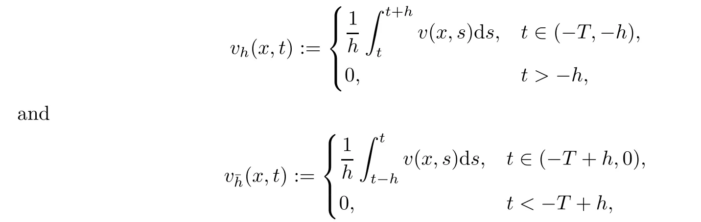


2.4 Minimizing affine function


2.5 A-caloric approximation
3 Caccioppoli Type Inequality

4 Poincar Type Inequality


5 Partial Regularity of u

5.1 Linearization

5.2 Decay estimate


6 Estimate of the Singular Set
6.1 Fractional time differentiability


6.2 Fractional space differentiability


 Acta Mathematica Scientia(English Series)2021年4期