Nonlinear Analysis and Applied Mathematics(NAAM)-Research Group,Department of Mathematics,Faculty of Science,King Abdulaziz University,P.O.Box 80203,Jeddah 21589,Saudi Arabia E-mail:bashirahmad qau@yahoo.com

Ravi P.AGARWAL

Department of Mathematics,Texas A&M University,Kingsville,Texas 78363-8202,USA E-mail:Ravi.Agarwal@tamuk.edu

Abrar BROOM Ahmed ALSAEDI

Nonlinear Analysis and Applied Mathematics(NAAM)-Research Group,Department of Mathematics,Faculty of Science,King Abdulaziz University,P.O.Box 80203,Jeddah 21589,Saudi Arabia E-mail:abrarbroom1992@gmail.com;aalsaedi@hotmail.com

Abstract By applying the standard fixed point theorems,we prove the existence and uniqueness results for a system of coupled differential equations involving both left Caputo and right Riemann-Liouville fractional derivatives and mixed fractional integrals,supplemented with nonlocal coupled fractional integral boundary conditions.An example is also constructed for the illustration of the obtained results.

Key words Fractional differential equations;Caputo and Riemann-Liouville fractional derivatives;systems;existence;fixed point theorems

1 Introduction

In this paper,we discuss the existence of solutions for a coupled system of nonlinear fractional differential equations,involving both left Caputo and right Riemann-Liouville fractional derivatives and mixed fractional integrals,equipped with nonlocal coupled fractional integral boundary conditions.In precise terms,we investigate the following system:

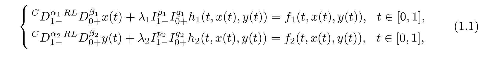
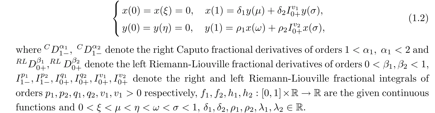
subject to integral boundary conditions:

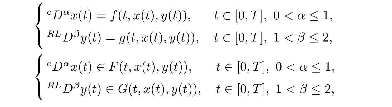
Before proceeding further,let us dwell some recent advancement in the study of fractional-order boundary value problems.The literature on the topic mainly deals with Caputo,Riemann-Liouville and Hadamard type fractional derivatives;for instance,see the texts[2–4]and articles[5–12].Fractional differential systems appear in the mathematical modeling of many real-world problems[13–15].For theoretical treatment of such systems,we refer the reader to the papers[16–18]and the references cited therein.In a recent article[19],the authors discussed the existence of solutions for the following systems of Caputo and Riemannn-Liouville type mixed order coupled fractional differential equations and inclusions:

subject to the boundary conditions:

x

(0)=

λ

D

y

(

η

)

,y

(0)=0

,y

(

T

)=

γI

x

(

ξ

)

,λ,γ

∈R

,η,ξ

∈(0

,T

)

,

where

D

,

D

are the Caputo fractional derivatives of order

α

and

p

∈(0

,

1)respectively,

D

is the Riemann-Liouville fractional derivatives of order

β,I

is the Riemann-Liouville fractional integral of order

q>

0

,f,g

:[0

,T

]×R×R→R

,F,G

:[0

,T

]×R×R→P(R)are the given continuous functions,and P(R)is the family of all nonempty subsets of R

.

On the other hand,boundary value problems of differential equations involving both left and right fractional derivatives of different orders and fractional integrals need further attention in view of the importance of these equations in the study of variational principles and Euler–Lagrange equations[20].In a recent article[21],the authors used the left-sided and rightsided fractional derivatives to formulate the fractional diffusion-advection equation related to anomalous superdiffusive transport phenomena.One can find some recent results on this class of boundary value problems in the articles[22–25].

The rest of this paper is organized as follows:in Section 2,we prove an auxiliary lemma,which plays a key role in converting the given problem to a fixed-point problem.Main results for our problem,presented in Section 3,are proved by means of Krasnoselskii’s fixed point theorem and contraction mapping principle.This paper concludes with illustrative examples.

2 An Auxiliary Lemma

Before presenting an auxiliary lemma,we recall some related de finitions from fractional calculus[2].

De finition 2.1

The left and right Riemann-Liouville fractional integrals of order

β>

0 for

g

∈

L

[

a,b

]

,

existing almost everywhere on[

a,b

]

,

are respectively de fined by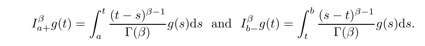

Lemma 2.2

For

g

∈

L

[

a,b

]

,

1≤

p<

∞and

q

,q

>

0,the following relations hold almost everywhere on[

a,b

]:

Of course,if

g

∈

C

[

a,b

]or

q

+

q

>

1,then the above relations hold for each

x

∈[

a,b

]

.

De finition 2.3

For

g

∈

AC

[

a,b

]

,

the left Riemann-Liouville and the right Caputo fractional derivatives of order

β

∈(

n

?1

,n

]

,n

∈N

,

existing almost everywhere on[

a,b

]

,

are respectively de fined by

In the following lemma,we solve a linear variant of system(1.1)–(1.2).

Lemma 2.4

Let

F

,F

,H

,H

∈

C

([0

,

1]

,

R).Then,the unique solution of the linear system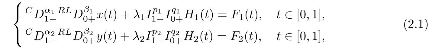

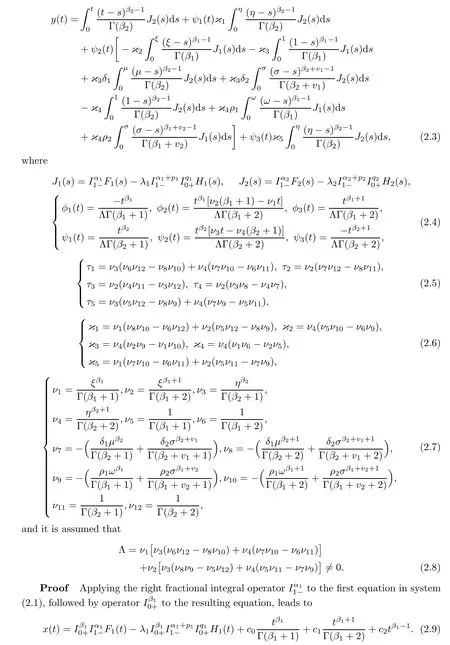
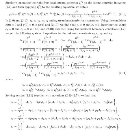
subject to the boundary conditions(1.2)is given by

where Λ is given by(2.8).Inserting the values of

c

,c

,c

,c

,c

and

c

in(2.9)and(2.10)and using the notations(2.4),we get solutions(2.2)and(2.3).The converse follows by direct computation.This completes the proof.

3 Main Results

Let X=

C

([0

,

1]

,

R)denote the Banach space of all continuous functions from[0

,

1]→R equipped with the norm‖

x

‖=sup{|

x

(

t

)|:

t

∈[0

,

1]}

.

The product space(X×X

,

‖(

x,y

)‖)is also Banach space endowed with norm‖(

x,y

)‖=‖

x

‖+‖

y

‖

.

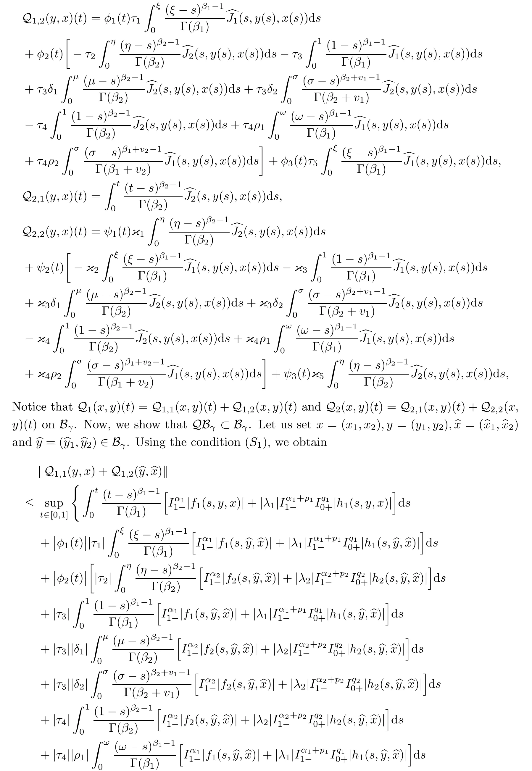
In view of Lemma 2.4,we de fine an operator Q:X×X→X×X as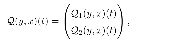

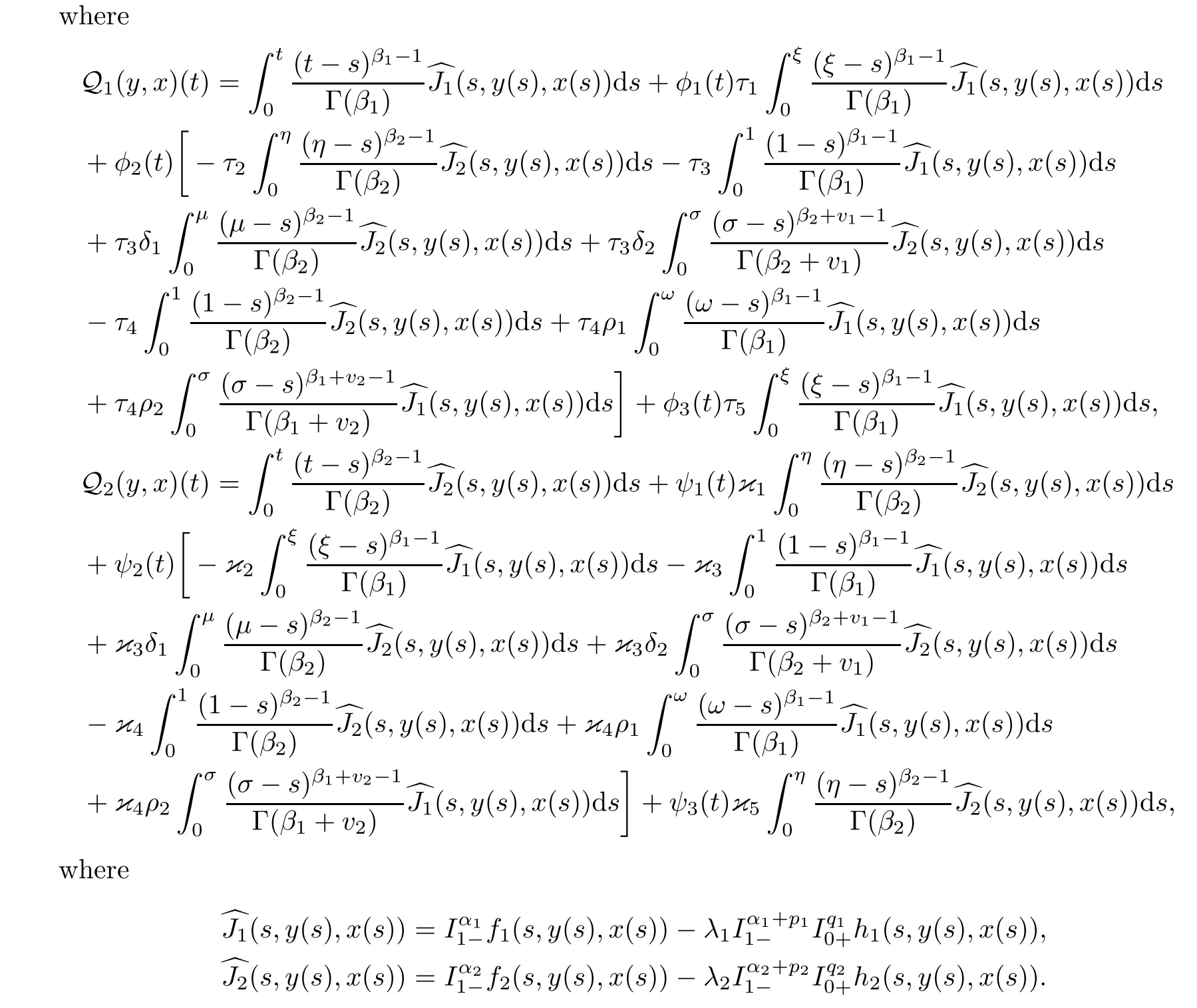
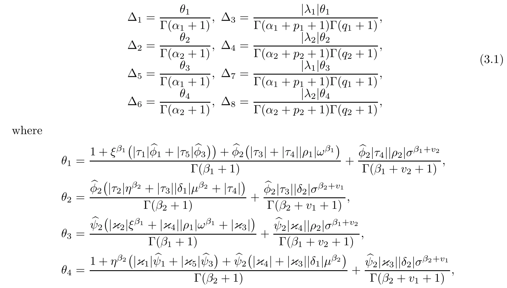
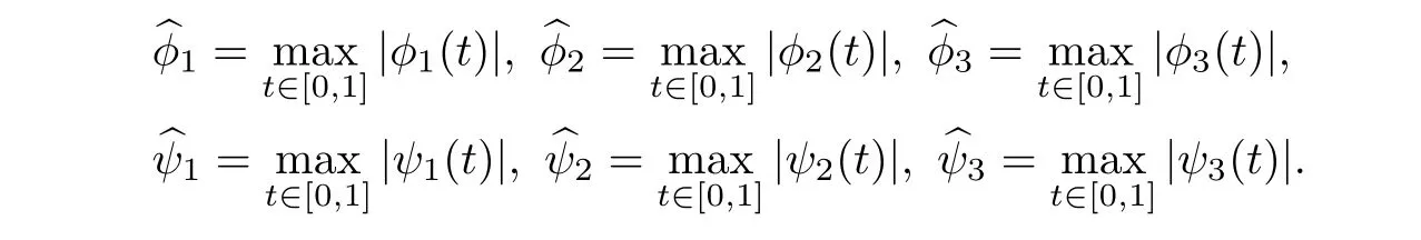
For computational convenience,we set

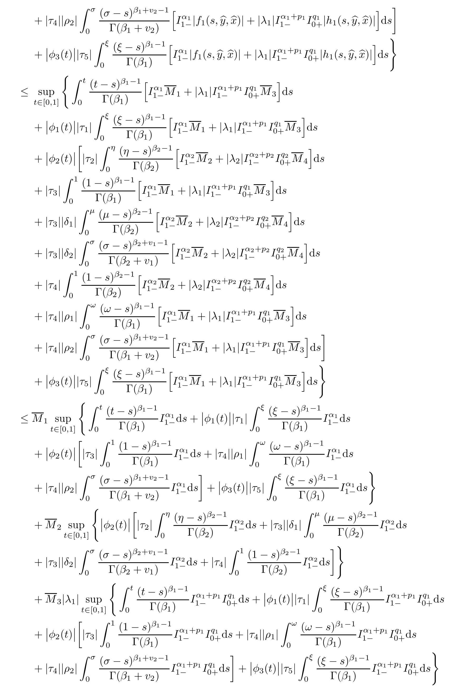
In the sequel,we need the following assumptions:

(

S

)Let

f

,h

:[0

,

1]×R×R→R(

i

=1

,

2)be the real valued continuous functions such that,for all

t

∈[0

,

1]and

x,y

∈R,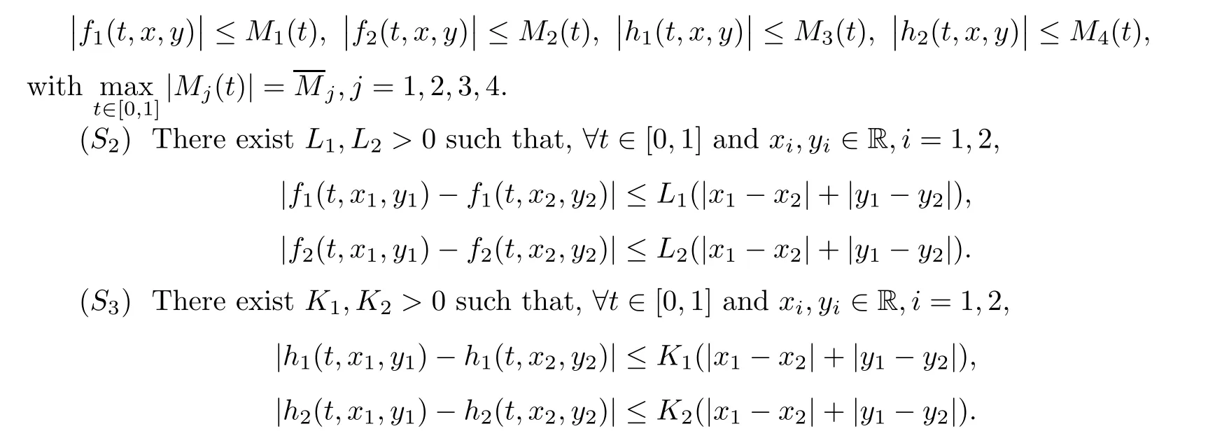

In the following theorem,we prove an existence result for system(1.1)–(1.2)via Kras-noselskii’s fixed point Theorem.For the reader’s convenience,we provide the statement of Kras-noselskii’s fixed point Theorem below.

Lemma 3.1

(Krasnoselskii[26])Let X be a closed,hounded,convex and nonempty subset of a Banach space у.Let H,Hbe operators mapping X to у such that(a)H

z

+H

z

∈X for

z

,z

∈X;

(b)His compact and continuous;

(c)His a contraction mapping.

Then there exists

z

∈X such that

z

=H

z

+H

z

.

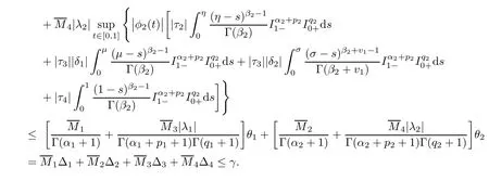
Theorem 3.2

Suppose that(

S

),(

S

)and(

S

)hold.Then,system(1.1)–(1.2)has at least one solution on[0

,

1]provided that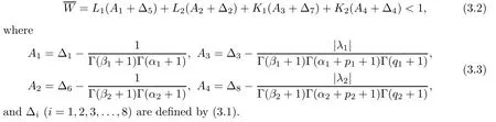

Proof

Introduce a closed,bounded and convex subset of X×X as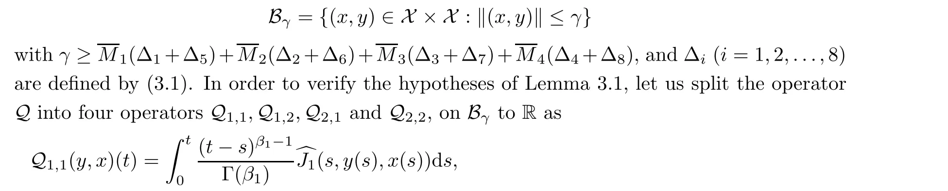

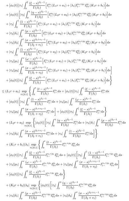
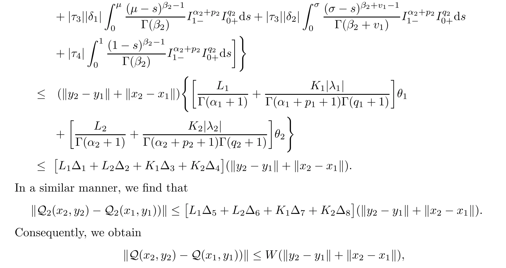
Similarly,we can find that

Now we prove that the operator(Q,Q)is a contraction by using the conditions(

S

)and(

S

).For(

x

,y

)

,

(

x

,y

)∈B,we have that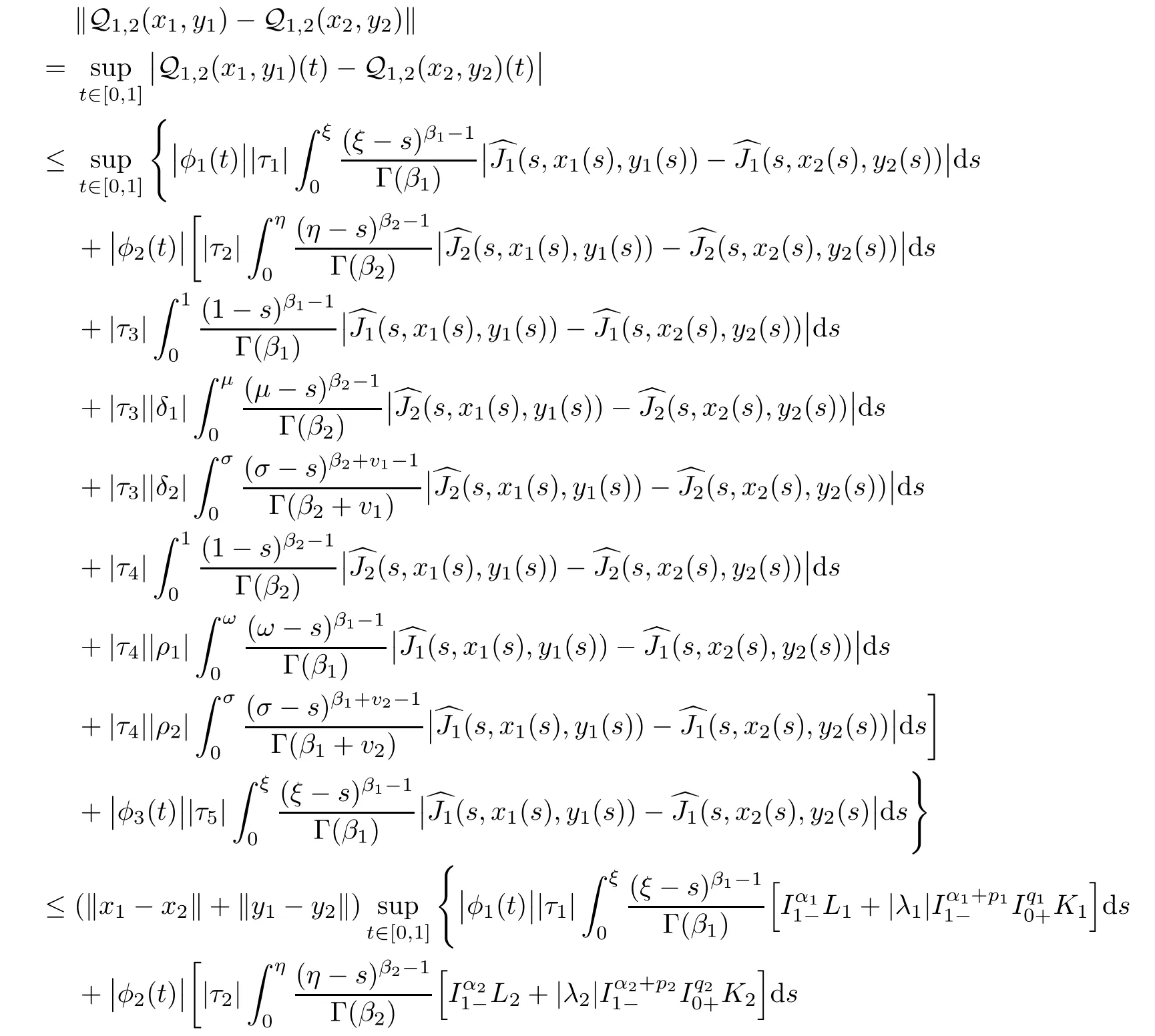

Likewise,we can obtain

From(3.4)and(3.5),we deduce that

which,by assumption(3.2),implies that the operator(Q,Q)is a contraction.Next,we show that the operator(Q,Q)is compact and continuous.By continuity of the functions

f

,f

,h

,h

,the operator(Q,Q)is continuous.For(

x,y

)∈B,we have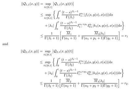

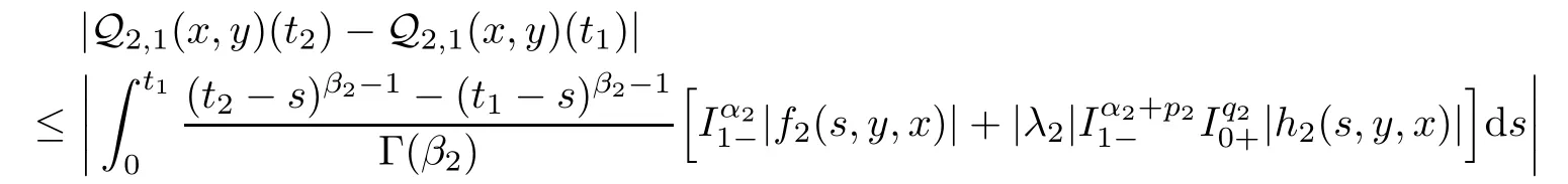
In consequence,we have

Therefore,the operator(Q,Q)is uniformly bounded on B.Next we show that(Q,Q)is equicontinuous.For 0

<t

<t

<

1 and?(

x,y

)∈B,we obtain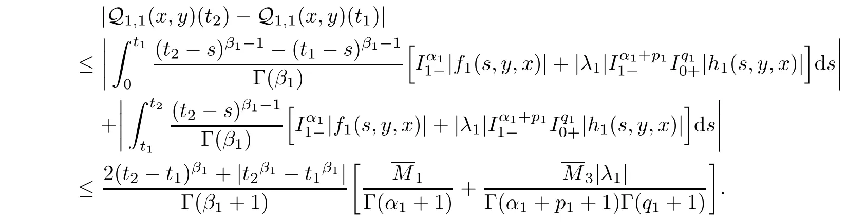

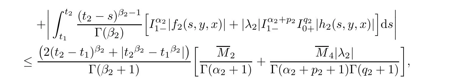
Analogously,we can find that

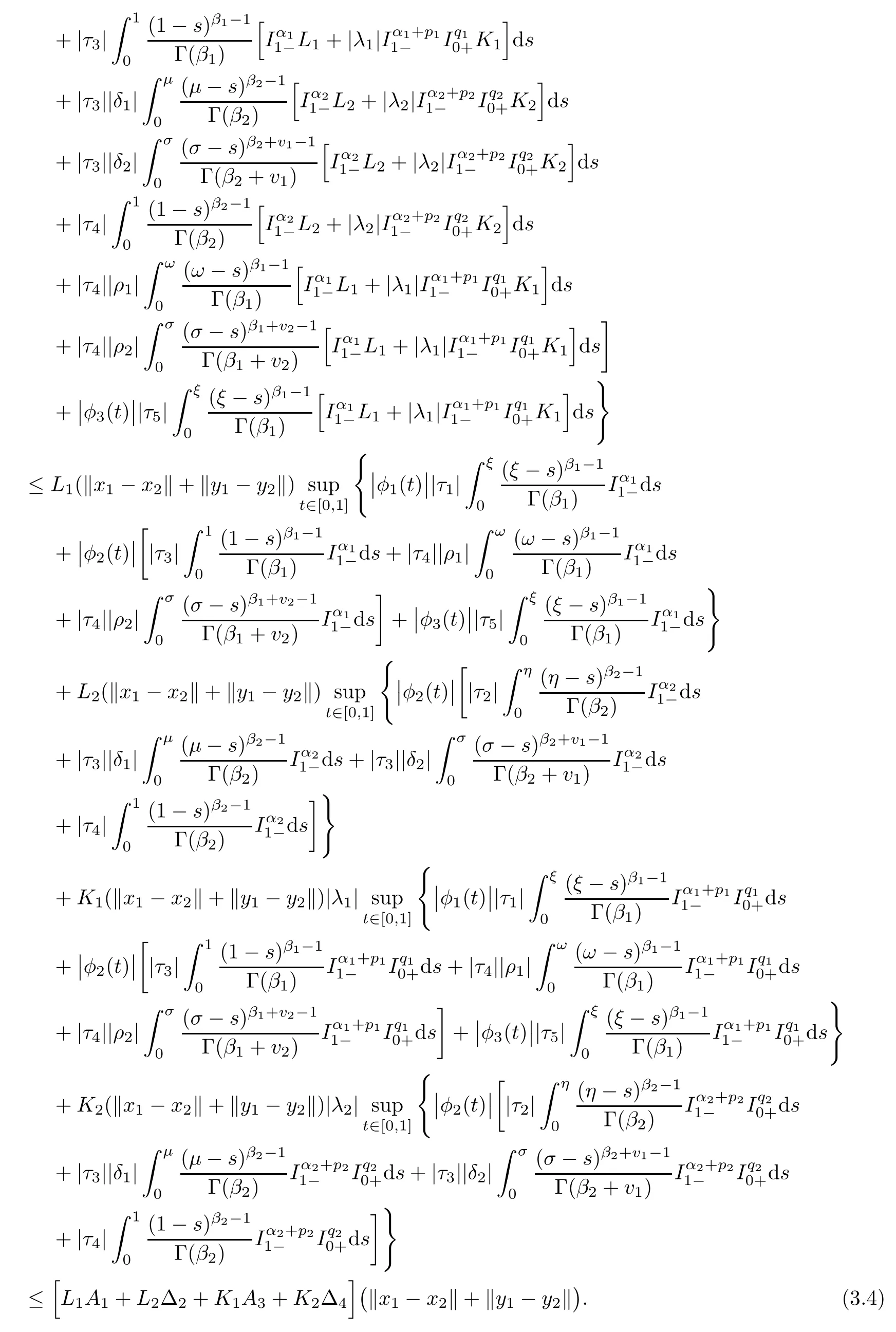
Now,we prove the uniqueness of solutions for system(1.1)–(1.2)via the Banach contraction mapping principle.

Theorem 3.3

Let

f

,f

,h

,h

:[0

,

1]×R×R→R be continuous functions satisfying assumptions(

S

)and(

S

).Then,problem(1.1)–(1.2)has a unique solution on[0

,

1]if

W<

1

,

where

and?(

i

=1

,

2

,...,

8)are de fined by(3.1).

Proof

Let us fix a positive number

r

such that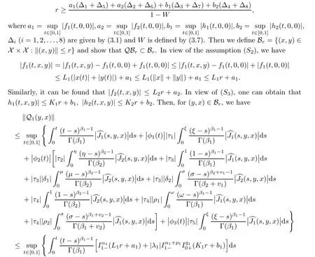

‖Q(

x,y

)‖≤

Wr

+(?+?)

a

+(?+?)

a

+(?+?)

b

+(?+?)

b

<r,

which implies that Q(

x,y

)∈Bfor any(

x,y

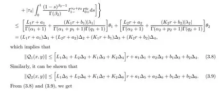
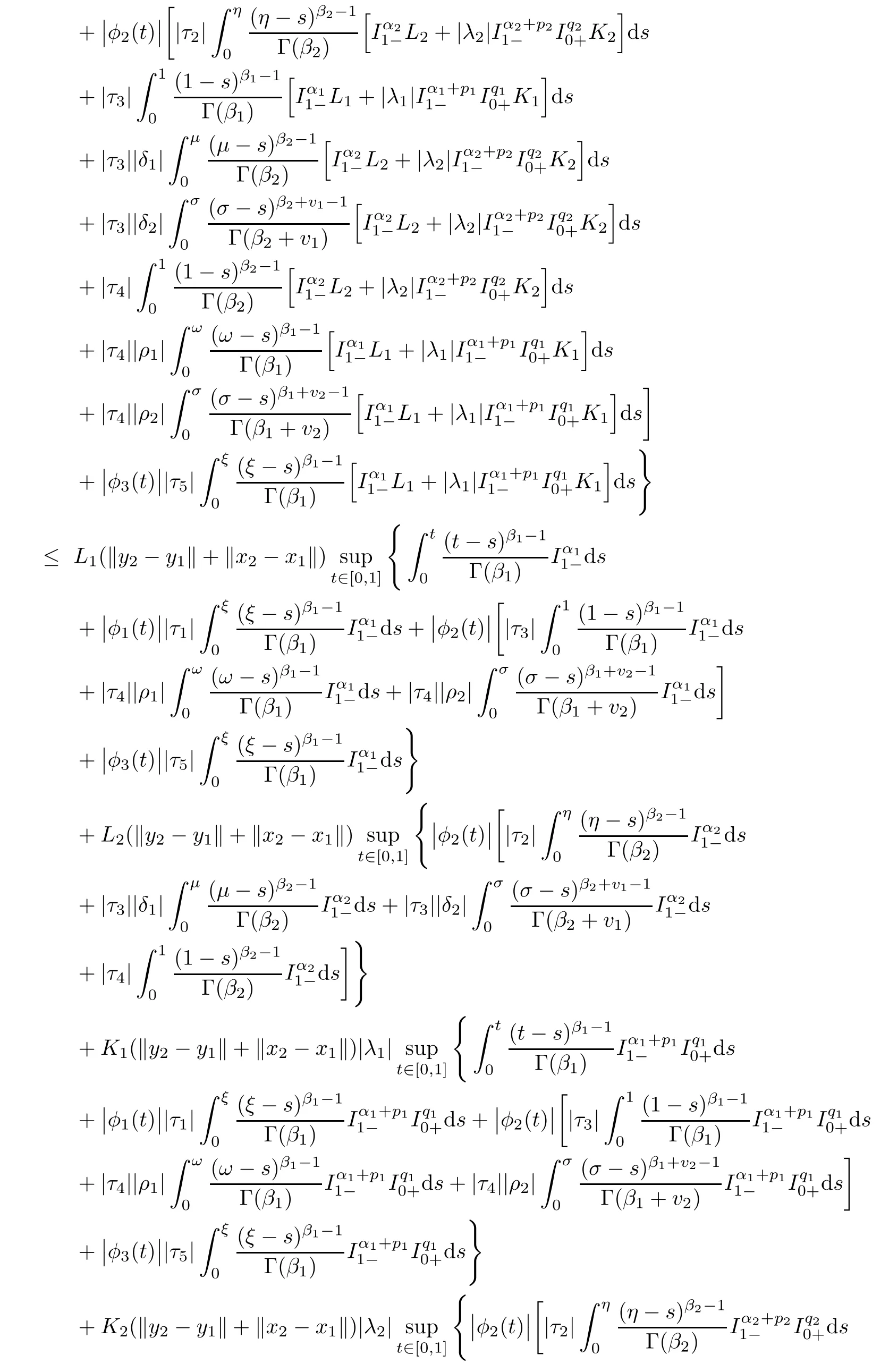
)∈B.Therefore QB?B.Now,we prove that Q is a contraction.Let(

x

,y

)

,

(

x

,y

)∈X×X for each

t

∈[0

,

1]

.

Then,by the conditions(

S

)and(

S

),we obtain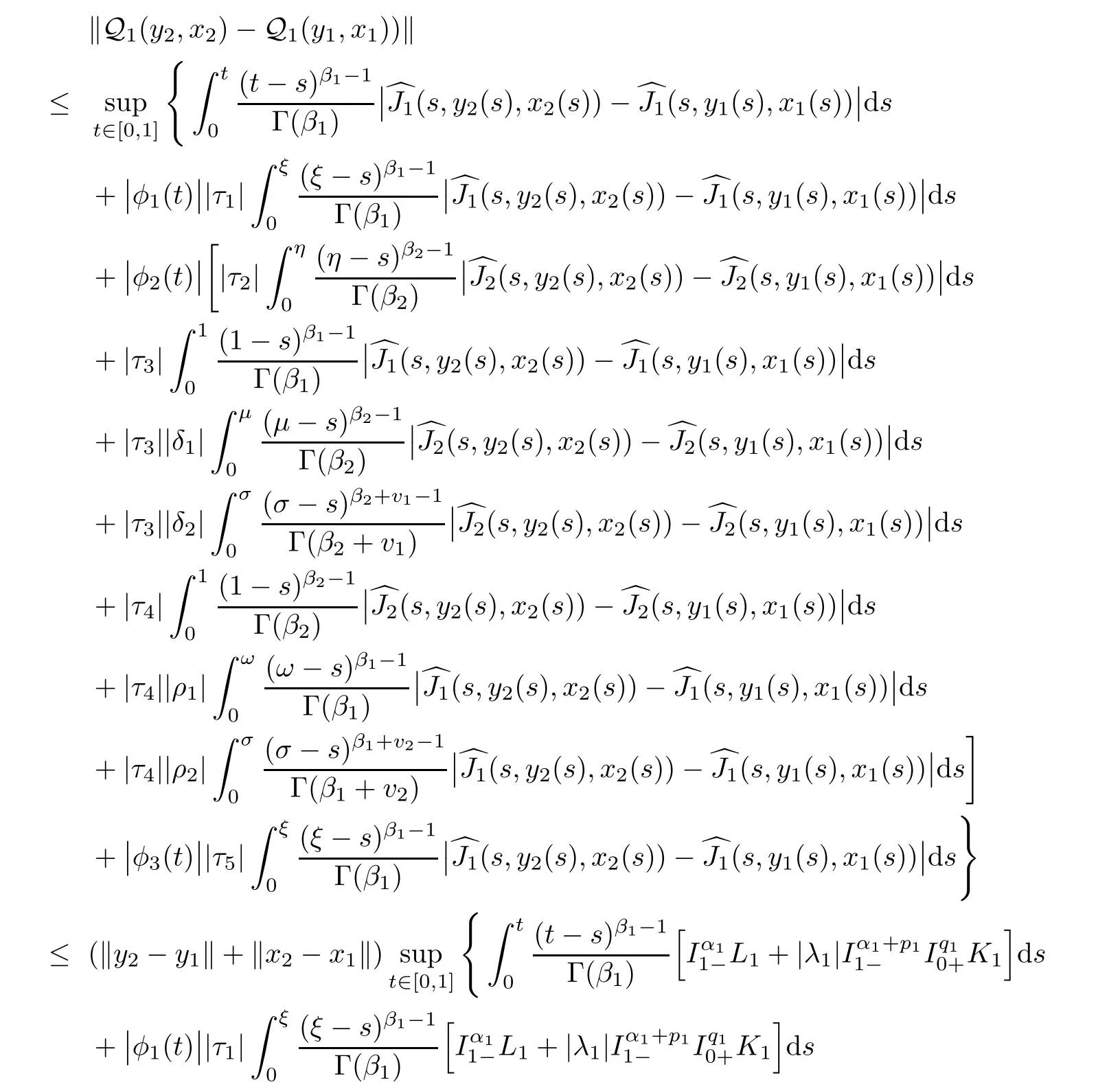

which,in view of the assumption

W<

1

,

implies that Q is a contraction.Hence it follows by Banach fixed point theorem that the operator Q has a unique fixed point,which corresponds to a unique solution of problem(1.1)–(1.2)on[0

,

1]

.

The proof is finished.

4 Example

Consider a coupled system of fractional differential equations containing Caputo and Riemann-Liouville derivatives of fixed orders and supplemented with coupled fractional integral boundary conditions given by

where

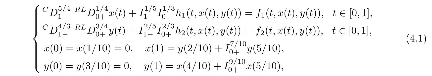
α

=5

/

4

,α

=4

/

3

,β

=1

/

4

,β

=3

/

4

,p

=1

/

5

,p

=2

/

5

,q

=1

/

3

,q

=2

/

3

,λ

=

λ

=1

,δ

=

δ

=

ρ

=

ρ

=1

,ξ

=1

/

10

,μ

=2

/

10

,η

=3

/

10

,ω

=4

/

10

,σ

=5

/

10

,v

=7

/

10

,v

=9

/

10

,

Observe that(

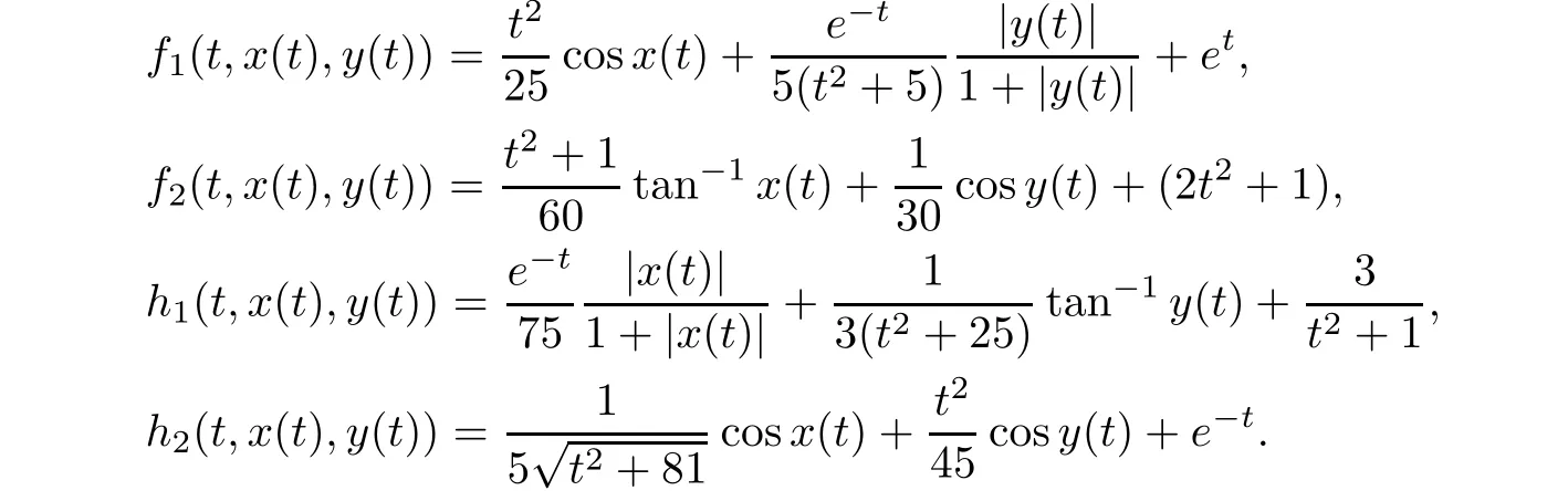
S

)is satisfied because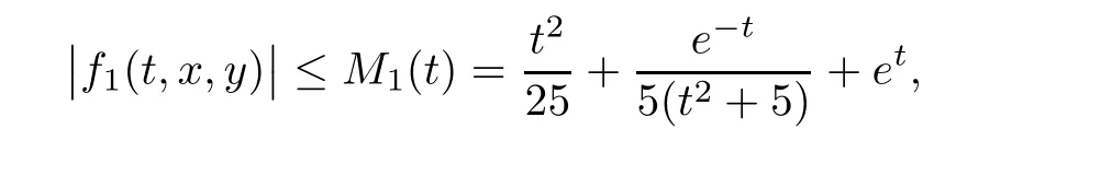

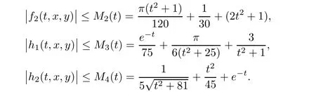
One can easily verify that conditions(

S

)and(

S

)are satis fied with

L

=1

/

25

,L

=1

/

30

,K

=1

/

75

,

and

K

=1

/

45

.

With the given values,we find that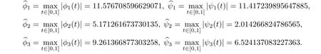

Furthermore,the values of Λ(given by(2.8)and?

,i

=1

,

2

,...,

8(de fined by(3.1))are found to be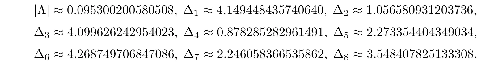

Using the given values,we get

where

A

=3

.

175697653501054

,A

=3

.

354900140842817

,A

=3

.

137567231307605

,

and

A

=2

.

788768311529850

.

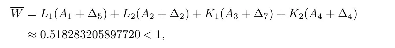
Thus,all the conditions of Theorem 3.2 are satis fied and consequently,its conclusion applies to system(4.1).Also,

W

≈0

.

617403220956142

<

1

,

where

W

is de fined by(3

.

7).Thus,the hypothesis of Theorem 3.3 is satisfied and hence its conclusion ensures that there exists a unique solution for system(4.1)on[0

,

1].

Acknowledgements

This project was funded by the Deanship of Scienti fic Research(DSR),King Abdulaziz University,Jeddah,Saudi Arabia under grant no.(KEP-MSc-63-130-42).The authors,therefore,acknowledge with thanks DSR technical and financial support.