
Quantum annealing for semi-supervised learning
2021-05-06 08:56:36YuLinZheng鄭玉鱗WenZhang張文ChengZhou周誠andWeiGeng耿巍
Chinese Physics B 2021年4期
關鍵詞:張文
Yu-Lin Zheng(鄭玉鱗), Wen Zhang(張文), Cheng Zhou(周誠), and Wei Geng(耿巍)
Hisilicon Research,Huawei Technologies Co.,Ltd.,Shenzhen,China
Keywords: quantum annealing,semi-supervised learning,machine learning
1. Introduction
The recent developments of machine learning enable computers to infer patterns that were previously untenable from a large data set.[1,2]Quantum computing, on the other hand, has been proved to outperform classical computers in some specific algorithms.[3–7]To extend both advantages, increasing efforts have been made to explore the merging of these two disciplines.[8–10]For instance, the quantum version of linear models of machine learning, such as support vector machines(SVM),[11]principal component analysis(PCA),[12]can be potentially more efficient than their classical versions.Quantum generative models were also proposed with exponential speedups compared to the traditional models.[13]However, most of those algorithms require a large-scale faulttolerant quantum computer that is beyond the ability of current hardware techniques.
Meanwhile, quantum annealer, as one of the noisyintermediate scale quantum (NISQ) devices,[14]has been proved useful in many applications such as optimization,[15]simulation,[16]and machine learning.[17]In this work,we propose a method to tackle semi-supervised classification tasks on a quantum annealer. An encoding scheme and a similaritycalculation method that map the graph representation of the problem to the Hamiltonian of a quantum annealing(QA)system are suggested, which avoid the implementation of multiqubit interaction. We show in two examples that good classification accuracy can be achieved using only a small amount of labeled data.
1.1. Semi-supervised learning
1.2. Quantum annealing
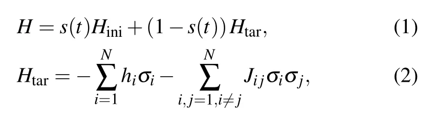
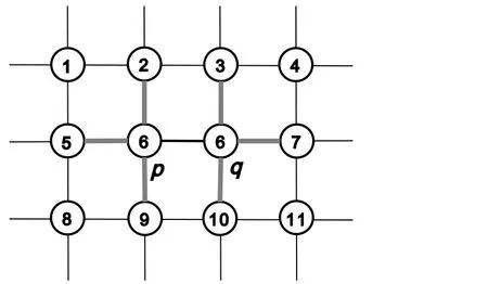
In a QA process,[27]the system is firstly prepared in a ground state of an initial Hamiltonian. A target Hamiltonian is gradually applied to the system as it evolves following the time-dependent Schr¨odinger equation.If the application of the target Hamiltonian is slow enough, the system will adiabatically stay at the ground state of the instantaneous Hamiltonian and finally reach to the ground state of the target Hamiltonian,which encodes the solution of the problem. Demonstration of QA has been vastly reported using systems based on superconducting circuits.[28–31]When an Ising model is used in a QA system, the Hamiltonian of the annealing process is usually defined as below:
2. Method
In this section,we introduce the whole procedures of our algorithm,as illustrated in Fig.1.
2.1. Label encoding
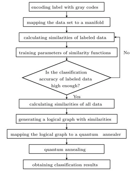
Fig.1. A flowchart of our method.
Generally,we can calculate the centers of each label with the aid of distribution assumptions for different labeled data sets. For example, if the data set of a particular label is big enough and follows a particular normal distribution, we can calculate its center with a better accuracy than the barycenter.
Though the complexity of finding the shortest path in the manifold is equivalent to the well-known travelling salesman problem, in most cases, the number of label is far fewer than that of data in a given data set. If the number of label is too large to endure while solving by a classical computer,we can also apply a quantum annealer to the problem. It has also been shown that this kind of task could also be potentially accelerated by a QA device.[35]
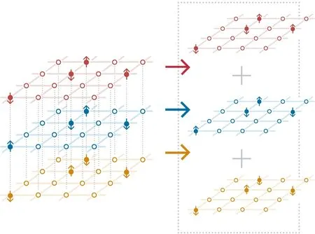
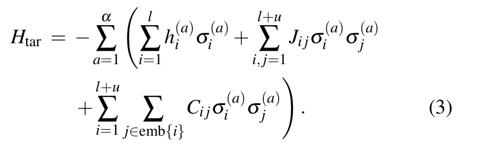
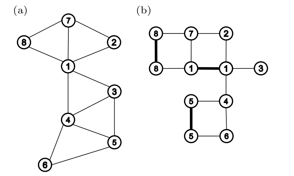
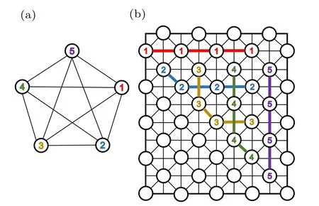
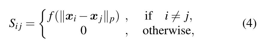
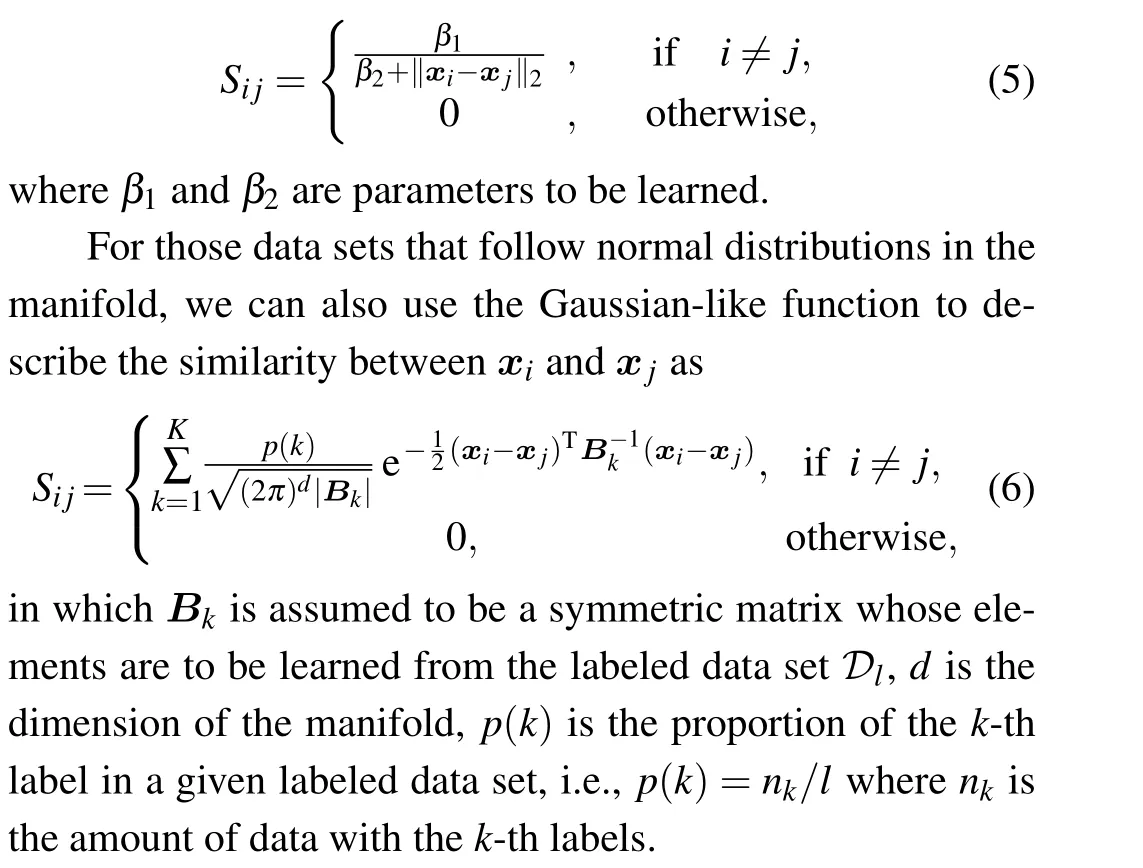
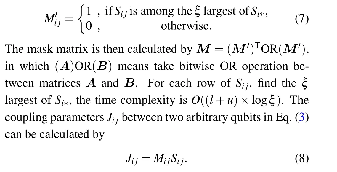
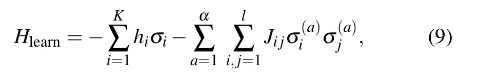
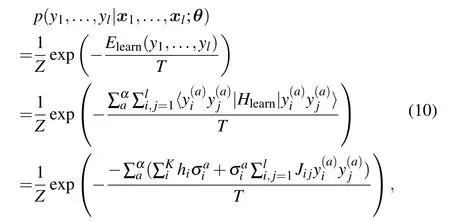
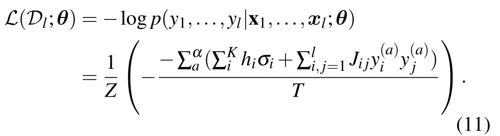
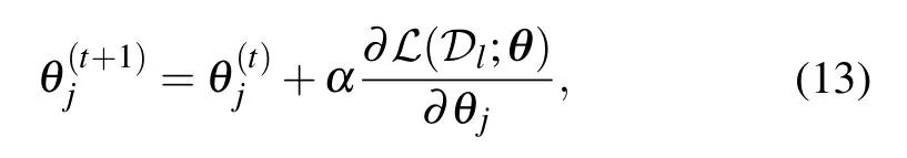
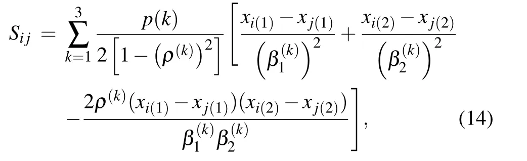
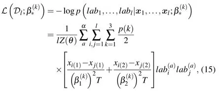
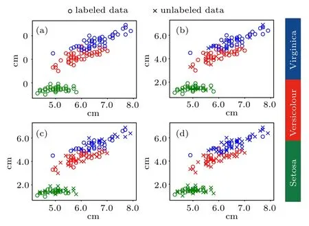
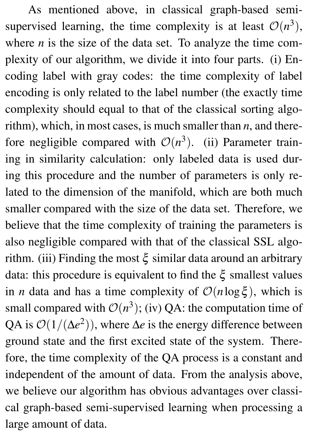
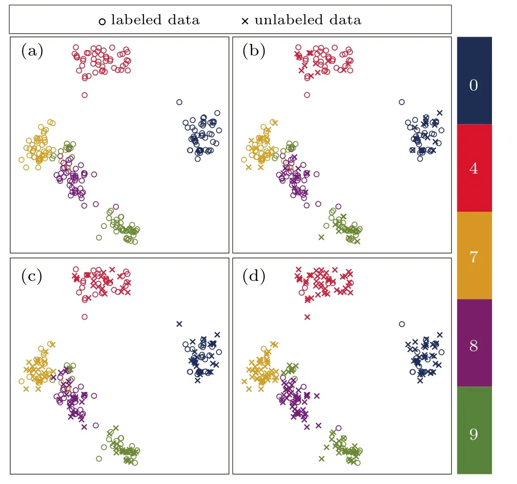
There are certainly cases that 2α?1 This system can naturally lead to a time-division multiplexing manner,such that each part of the training process can be operated separately in time using just one smaller system.This is especially advantageous when the number of qubits in a QA hardware is limited compared with the problem size. In fact,such a time-division multiplexing manner is equivalent to a dichotomy method, that is, by determining each bit of the binary label code,the total unlabeled data are sorted into two groups after each annealing process. An example of such a system is delineated in Fig.2. Moreover,we specify two configurations for labeled and unlabeled data separately: Labeled dataTo assure that the qubits of labeled data reveal correct labels after being measured at the end of the annealing process,we should apply a bias hithat is large enough to make the probability of their transition to wrong states close to 0 at the end of the QA process. Fig.2. Example of the QA structure that performs the SSL classification task. Each qubit, depicted in the solid or open circle, expresses one bit of the label code of a labeled or unlabeled data,respectively. A group of three qubits connected with a dashed line represents one data. Arrows on the labeled data indicate the directions of hi on corresponding qubit qi. In this example, each qubit in the same layer is topologically coupled with its 4 neighbors. A time-division multiplexing scheme can be used by dividing the system in to 3 smaller systems that are annealed individually. Unlabeled dataNo bias is applied to the corresponding qubits. Hence,Eq.(2)can be re-written as Fig.3. An example of the connecting method that increases number of connections between qubits. Circles represent physical qubits and solid lines are physical couplings between two qubits. Each qubit is physically connected to its four surrounding qubits. The thicker lines represent a maximal coupling Cpq between qubits p and q, such that they could be treated as a single data qubit denoted as y6. As a result,6 qubits(i.e.,y2,3,5,7,9,10)are logically connected to y6. Fig.4. Mapping a graph to qubits in square lattices. (a)The original graph to be mapped on a quantum annealer. (b)A way to connect physical qubits in square lattices to represent the graph shown in(a).The thick lines indicate that the qubits on the ends of the lines are maximally coupled. In extreme cases,we can map an all-connected graph to a quantum annealer by King’s graph as shown in Fig.5.[36,37] Fig.5. (a) The original graph with full connection of 5 qubits. (b) An example for a connecting method on a quantum annealer with King’s graph corresponding to the graph shown in(a). In the QA model of Eq.(3),when Jij>0,the stronger the two qubits are coupled, the more likely they are to have the same orientations. Therefore,it is intuitive to map the similarity between two data to the coupling coefficient between two qubits in a QA system. According to the vectors of two data in the manifold,the similarity between the two data can be calculated as below: where‖Θ‖pis the p-norm of vector Θ and f(Θ)is a monotonically decreasing function of Θ. To better describe the similarities of a particular data set, f(Θ)may contain parameters that can be learned. For example,we can use Euclidean distancebased similarity It should be noted that in this step, similarities between unlabeled data are also calculated,as we find out that the density information hidden in unlabeled data is also helpful during the QA process. In the final step,we attribute appropriate values to the parameters that are related to the system’s Hamiltonian. Firstly,the parameters involved in the similarity calculation can be determined by a supervised learning process using the labeled data set. In the learning process,we have A negative log-likelihood function is therefore defined as below: The iterative strategy is as follows: in which α is the learning rate which controls the step of each round,and the gradient term can be easily calculated by sampling the annealing result. While the number of parameters is small,we can also traverse all the possible values. Such a learning process is similar with the Boltzmann machine model,[33,38,39]except that the sampling process can be accelerated by iterated QA processes and project measurements of qubits.[17] Here we give two examples based on realistic database to verify the method discussed above. As a proof-of-principle demonstration, the annealing processes are simulated by a classical computer. It should be noted that a quantum annealer may exhibits control errors such that the actual connection coefficient is not exactly what we have calculated. So when we simulate the protocol on the classical computer,we add a random disturb about 3%on{hi},{Jij},and{Cij}. We first use a database of iris that has been widely used in pattern recognition literature.[40]There are three kinds of label in the data set,shown by points in three colors in Fig.6(a).According to the labeled data(open circles),it is obvious that the shortest path that connects all the labels’barycenters is green–red–blue. Therefore,we encode the label by an ordered binary gray code as {00}Setosa, {01}Versicolour, and {10,11}Virginica.We assume that the similarity between arbitrary two data follows a 2-dimensional mixed Gaussian-like function The classification results are shown in Figs. 6(b)–6(d).When 30% of the data set is unlabeled, the accuracy of the algorithm is 100%. An accuracy of 94.26%can still be maintained when 80%unlabeled data is considered. Fig.6. The original iris data set (a) and the classification results using the algorithm proposed in this work when the portion of unlabeled is (b) 30%with 97.89%accuracy rate,(c)50%with 94.44%accuracy rate,and(d)80%with 96.26%accuracy rate. The circles in the picture represent labeled data and the crosses represent unlabeled data. The y axis of the graph is the petal length in cm and the x axis is the sepal length in cm. The second example is the handwritten digital recognition using the database from MNIST. We pick 250 pieces of 8×8 pixels images of digits 0, 4, 7, 8, and 9 from the original data set and reduce the original dimension to 2 by Isomap function as shown in Fig.7(a). According to their barycenters on the manifold,we encode the 4 labels by{000,100}0(blue),{001}4(red), {011,010}7(yellow), {111,101}8(purple), and{110}9(green). Fig.7. The handwriting digits data set with reduced dimensions(a)and the digits 0,4,7,8,9 in blue,red,yellow,purple,and green,respectively. The classification results using the algorithm proposed in this work when the portion of unlabeled is(b)30%with 98.55%accuracy rate,(c)50%with 95.9%accuracy rate, and (d) 80% with 97.04% accuracy rate. The circuits in the picture represent labeled data and the crosses represent unlabeled data. Here the Euclidean distance given by Eq. (5) is applied to calculate the similarity matrix S and coupling parameters J, in which ξ =4 for 30%and 50%unlabeled and ξ =7 for 80%unlabeled data. In the simulation,we set the bias{hi}to 10. The parameters concerning the similarity calculation are trained using similar approaches as the first example. Figures 7(b)–7(d)show the classification results. The accuracy of QA-SSL changes from 96.15%to 92.13%as the portion of the unlabeled data in the whole data set increases from 30%to 80%,showing again the feasibility of this method. So far, quantum machine learning algorithms have been studied extensively on clustering (unsupervised learning)[34,42–44]or supervised learning classification algorithms.[11,45]In this paper we introduce a new semisupervised learning method based on QA. In this method,the classification problem is mapped to the QA Hamiltonian through a graph representation, of which the vertices are efficiently implemented by qubits with an encoding scheme based on a binary gray code. Calculations of the similarity between data are improved with a learning process using various models. Compared with previous proposed classification method using QA, this scheme significantly saves the quantum resources while maintaining the ability to express the original problem. The results of two proof-of-principle examples indicate that this method can still yield high accuracy for classification problem when the amount of labeled data is limited.2.2. Structure of the system
2.3. Similarity and coupling parameters

2.4. Parameters learning


3. Example
3.1. Example 1: iris

3.2. Example 2: handwriting digital pictures
4. Discussion
5. Conclusion
猜你喜歡
Chinese Physics B(2023年1期)2023-02-20 13:13:36
共產(chǎn)黨員·下(2022年4期)2022-05-17 02:10:08
Acta Mathematica Scientia(English Series)(2021年5期)2021-10-28 05:44:14
大觀·東京文學(2020年3期)2020-05-25 13:25:00
戀愛婚姻家庭(2019年10期)2019-11-04 06:11:37
歌海(2019年2期)2019-06-11 07:02:14
延河(下半月)(2019年4期)2019-04-23 06:47:40
戀愛婚姻家庭(2019年28期)2019-01-28 11:57:24
戲劇之家(2017年14期)2017-09-11 20:05:30
歌海(2017年6期)2017-05-30 05:20:26
- Chinese Physics B的其它文章
- Taking tomographic measurements for photonic qubits 88 ns before they are created*
- First principles study of behavior of helium at Fe(110)–graphene interface?
- Instability of single-walled carbon nanotubes conveying Jeffrey fluid?
- Relationship between manifold smoothness and adversarial vulnerability in deep learning with local errors?
- Weak-focused acoustic vortex generated by a focused ring array of planar transducers and its application in large-scale rotational object manipulation?
- Quantization of the band at the surface of charge density wave material 2H-TaSe2?