Qingquan TANG (唐清泉) Qiao XIN (辛巧) ?

College of Mathmatics and Statistics, Yili Normal University, Yining 835000, China

E-mail: xinqiaoylsy@163.com

Chunlai MU (穆春來)

College of Mathmatics and Statistics, Chongqing University, Chongqing 401331, China

E-mail: clmu2005@163.com

Abstract This article considers the following higher-dimensional quasilinear parabolic-parabolic-ODE chemotaxis system with generalized Logistic source and homogeneous Neu-mann boundary conditions in a bounded domain Ω ? Rn(n ≥ 2) with smooth boundary ?Ω, where the diffusion coef-ficient D(u) and the chemotactic sensitivity function S(u) are supposed to satisfy D(u) ≥M1(u + 1)?α and S(u) ≤ M2(u + 1)β, respectively, where M1,M2 ＞ 0 and α, β ∈ R. More-over, the logistic source f(u) is supposed to satisfy f(u) ≤ a ? μuγ with μ ＞ 0,γ≥ 1, and , we show that the solution of the above chemotaxis system with sufficiently smooth nonnegative initial data is uniformly bounded.

Key words Chemotaxis system; logistic source; global solution; boundedness

1 Introduction

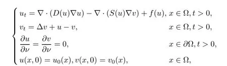
In this article, we consider the following quasilinear parabolic-parabolic-ODE chemotaxis system with generalized logistic source

in a bounded domain ? ?Rn(n ≥2) with smooth boundary ??.denotes the derivative with respect to the outer normal of ??. The diffusion coefficient D(u) and the chemotactic sensitivity S(u) are satisfying that

with M1>0 and α ∈R,

with M2>0 and β ∈R, as well as the logistic source f(u) is smooth satisfying f(0)≥0 and

with a ≥0, μ>0, and γ ≥1. For the nonnegative initial data, we assume that

The original model of chemotaxis system (1.1) was proposed by Strohm, Tyson, and Powell [1] to describe the aggregation and spread behavior of the Mountain Pine Beetle (MPB),u(x,t) denotes the density of the flying MPB, v(x,t) stands for the concentration of the beetle pheromone, and w(x,t) represents the density of the nesting MPB. The flying MPBs chew the tree body and make nests to lay eggs, the flying MPB can bias their movement according to concentration gradients of MPB pheromone,moreover,we also assume that the flying MPB are supposed to experience birth and death under a generalized logistic source. Different from the classical Keller-Segel chemotaxis model [2], the beetle pheromone, as a chemotactic cue only attracts the flying MPB,is secreted for the nesting MPB,and then,the chemotaxis model with indirect signal production, the generalized diffusion coefficient for the flying MBP and also the chemotactic sensitivity, are considered in this article. On the researches of the aggregation and spread behavior of MPB, Hu and Tao [3] proved that the solution of the chemotactic system(1.1) in 3D with D(u) = 1, S(u) = u, and γ = 2 was uniformly-in-time bounded. For the dimensional n ≥2, Qiu, Mu, and Wang [4] proved that the chemotaxis system, with S(u)=u and γ =2, had a unique global solution, and its solutions was also uniformly-in-time bounded as α > 1 ?. Moreover, Li and Tao in [5] considered the system (1.1) with D(u) = 1 and S(u) = u, and the global existence and boundedness of smooth solutions to this system was obtained as γ >. In this article, the generalized diffusion coefficient will be considered for the flying MBP and also the generalized chemotactic sensitivity function.

The main idea and methods of this article come from the work of Zhang and Li [6], they considered the following quasilinear fully parabolic Keller-Segel system with logistic source

where D(u)≥M(u+1)?α, S(u)≤M(u+1)β, and f(u)≤a ?μuγwith γ ≥1 and n ≥1, andas

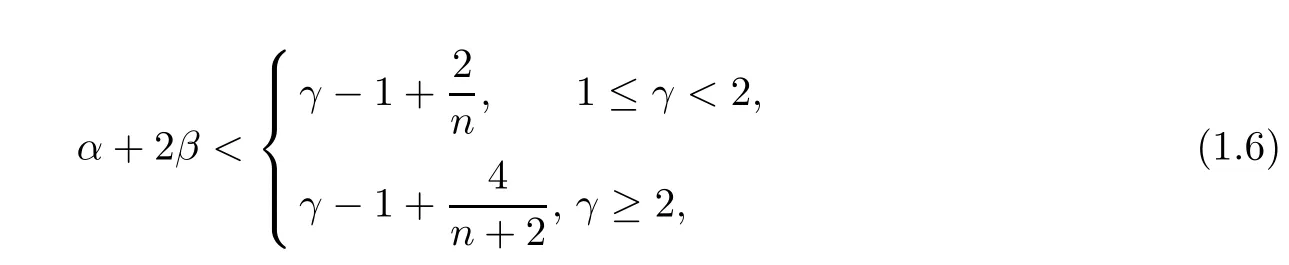
its solution was global and bounded under sufficiently smooth initial data. The nonlinearities like in (1.2) and (1.3) are originally from the so-called volume-filling effect derived by Hillen and Painter [7] and extended by Wang and Hillen [8]. Moreover, we should note that the chemotaxis system with terms (1.2) and (1.3) (without Logistic source) seem to be discussed first in the article by Wrzosek [11]; the relation between α + 2β ensuring the existence of solutions is obtained and further extended by Wang, Winkler, and Wrzosek [10]. About the boundedness, Blow-up, asymptotic behavior of the solution to the Keller-Segel model which maybe quasilinear,degenerated,singular,the readers can refer to[11–15]and also the reference therein. Similar to the discussions in [6], the first focus of this article is also to provide more details on the interaction of the competing mechanisms for the self-diffusion, cross-diffusion in the chemotaxis system (1.1), this is described by the parameter α+2β from the perspective of mathematics; moreover,we also consider the role of the generalized Logistic source,that is the parameter γ. Furthermore, we obtain the following main results.

Theorem 1.1Let ? ?Rn(n ≥2) be a bounded domain with smooth boundary ?? and the hypothesis (1.2)–(1.5) hold. As α+2β < γ ?1+, the quasilinear chemotaxis system(1.1) has a unique classical solution which is also global and bounded in ?×(0,∞).

Compared with the results for the chemotaxis system (1.1) which exist in the recent references, the current results can be considered as an extension of the corresponding results, and we have the following remarks.

Remark 1.2Observe the condition of Theorem 1.1 for the global boundeness of the solution to system (1.1). Firstly, setting n = 3, α = 0, β = 1, and γ = 2, Hu and Tao [3] got the global boundedness to the solution of system (1.1), and our conditionobviously holds. Moreover,letting α=?θ,β =1,and γ =2,Qiu,Mu,and Wang[4]obtain the global boundedness to the solution of system(1.1)as θ >1?,and this condition is coincident with ours. Finally, supposing α=0 and β =1,Li and Tao[5]obtained the global boundedness to the solution of system (1.1) as γ >for all n ≥2, and in the current hypothesis, our condition isbecause offor all n ≥4; thus, our results can be considered as an extension of the results in [5] in the case n ≥4.

Next, we propose the details for the proof of Theorem 1.1; we begin with some lemmas,which will be used in the following context.

2 Preliminaries

The local existence of the solution of the chemotaxis system (1.1) can be obtained by the standard way (Banach Fixed Point Theorem) of the parabolic-parabolic-ODE for taxis mechanisms, which is similar to the proof in [16, 17] and so on; we mainly have the following lemma.

Lemma 2.1Let D(u), S(u), and f(u) satisfy (1.2)–(1.5), respectively. Assume that u0∈C0, v0∈W1,ρwith ρ>max{2,n} and w0∈C0are non-negative function, and then, there exist Tmax∈(0,∞] and a unique triple (u,v,w) of non-negative function:

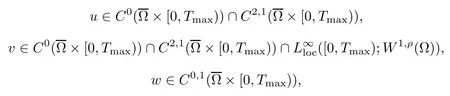
which solve the chemotaxis system (1.1) classically in ?×(0,Tmax); moreover, if Tmax< ∞,then

Next, the proof of the boundedness for the solution of the chemotaxis system (1.1) should begin with the elementary estimation of the solution u,v,w in Lp;we have the following lemma.

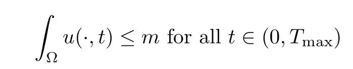
Lemma 2.2Let T ∈(0,Tmax), and then, there exists m > 0 and C > 0 such that the first component of the solution of the chemotaxis system (1.1) satisfies

and

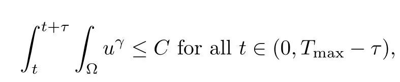
where

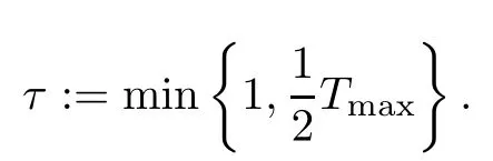
Furthermore, we obtain

ProofThe proof of this lemma is similar to Proofs of Lemmas 2.2 and 2.4 in [5], so we omit it here.

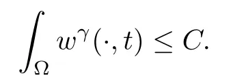
Remark 2.3If γ ≥n, then, we obtain

The proof can be found in [18]. Then, the following proof of Theorem 1.1 is easy to do, hence,we always assume that γ < n. Thus, in Lemma 2.1, as settingis meaningful, the proof can also be found in [18].

Remark 2.4The Lpboundedness of the solution v(x,t)is different to the corresponding result in [6]. The main reason maybe the existence of the ordinary differential equation on the nesting MPB in the chemotaxis system(1.1),and then,the chemotaxis system(1.1)may posses new properties which are different from the Keller-Segel models.

Moreover,the Gagliardo-Nirenberg inequality plays an important role in the following proof.For the details, we mainly refer to [19, 20].

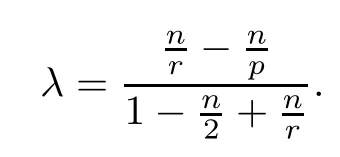
Lemma 2.5Let p ≥1,r ∈(0,p),and ψ ∈W1,2(?)∩Lr(?). Then,there exists a constant CGN>0 such that

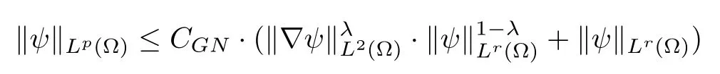
holds with λ ∈(0,1) and also satisfies

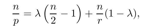
where

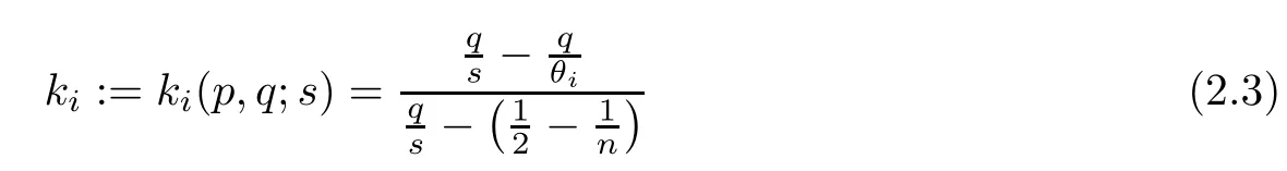
Using the Gagliardo-Nirenberg inequality, the suitable choosing of the parameters r and λ is very critical. Before this, we propose the choosing as follows. For any p ≥1, q ≥1, anddefine

and

Set

and

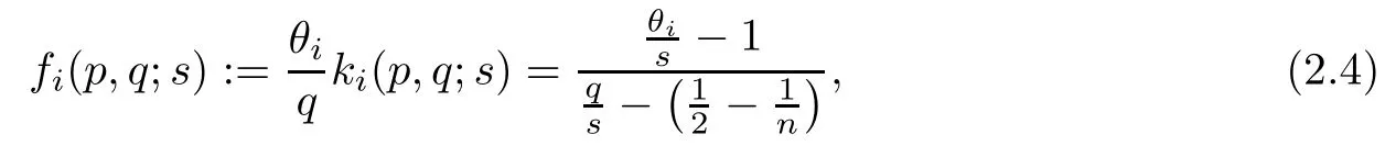
for i=1,2. Thus, we can obtain the following lemma on kiand fiunder suitable choosing p,q,where i=1,2.

Lemma 2.6For any sufficiently large p > 1,, andthere exists a number q >1 such that

ProofWe know that ki(p,q;s)∈(0,1) is equivalent to

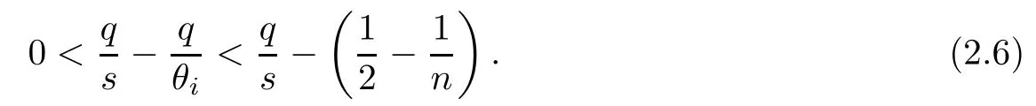
From the left hand of inequality (2.6), we can obtain θi>s. Moreover,for the right hand side of inequality (2.6), we obtain. On the other hand, fi(p,q;s) < 2 is equivalent to, that is. Because of θi>s, then we have

Thus, choose θi>s and, so that inequalities (2.5) hold. That is to say

is equivalent to equalities (2.5). By the definition of θiin (2.1) and 2.2, we can obtain

and

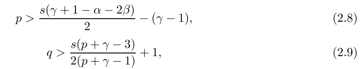
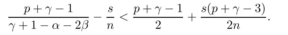
When p is large enough, inequality (2.8) holds. Moreover, as p > 1 andby the direct computation, it is easy to verify that

Now, q exists if and only if

3 A Bound for

We proceed to establish a crucial step towards the proof of the boundedness; that is establishing a bound forfor any p>1.

Lemma 3.1Let T ∈(0,Tmax) and the hypothesis (1.2)–(1.5) hold. Then, there exists C >0 independent of T such that the solution of chemotaxis system (1.1) fulfills

where θ1and θ2are defined as (2.1) and (2.2).

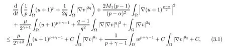
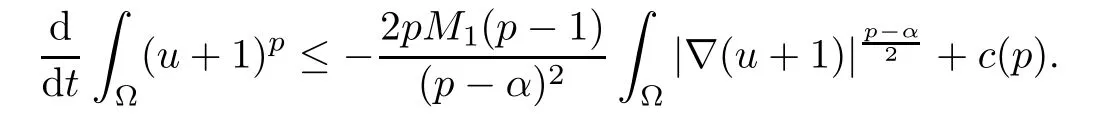
ProofUnder the assumption, the strong maximum principle entails u > 0 in× (0,Tmax). On the basis of this, we test the first equation in (1.1) by (u + 1)p?1and integrating over ?, then we obtain

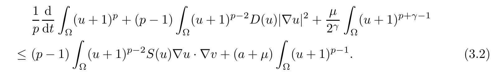
Here, because of (1.2), we obtain

From (1.3) and Young’s inequality, we obtain

and again using Young’s inequality,

Inserting (3.3)–(3.5) into (3.2) yields

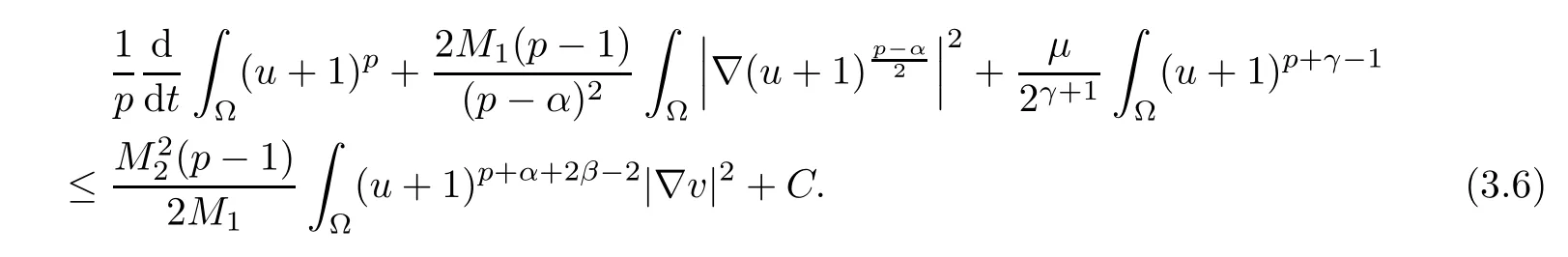
Next, using the second equation in (1.1), we obtain

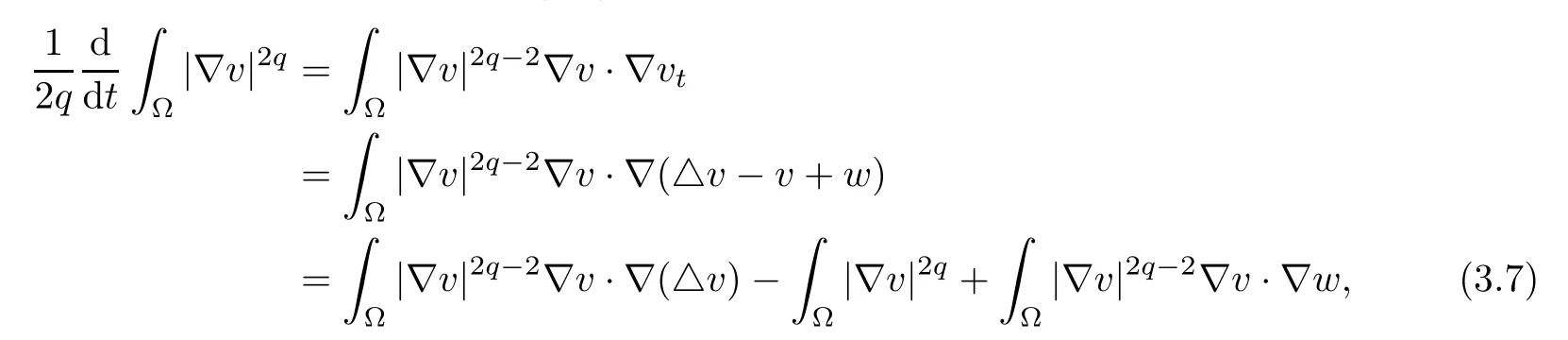
Invoking the identity △|?v|2=2?v·?(△v)+2|D2v|2, we obtain

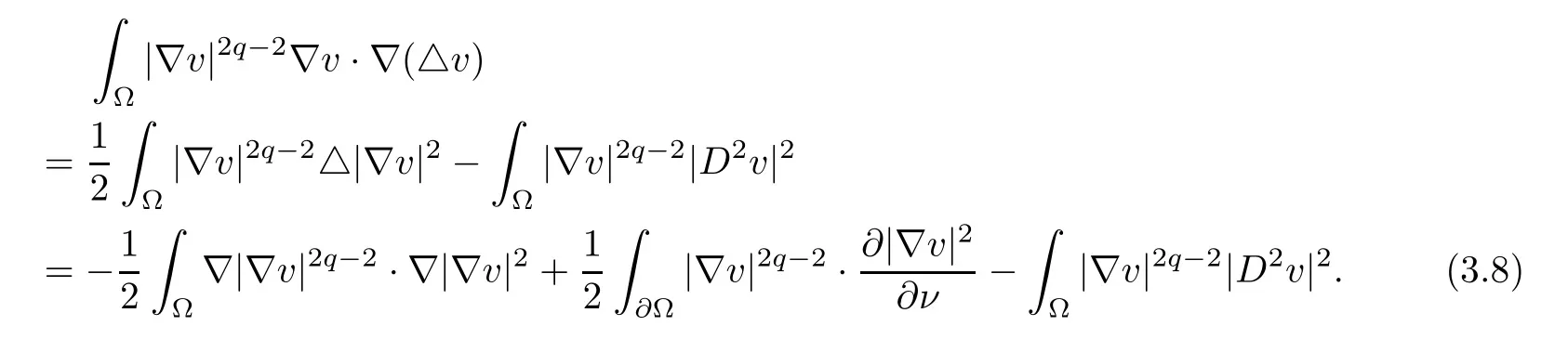
Because

and

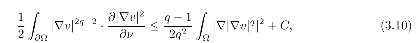
collecting (3.9)–(3.10) ensures that

Using Young’s equality, we obtain

because of |?v|2≤n|D2v|2. Together (3.7) with (3.11) and (3.12), we obtain

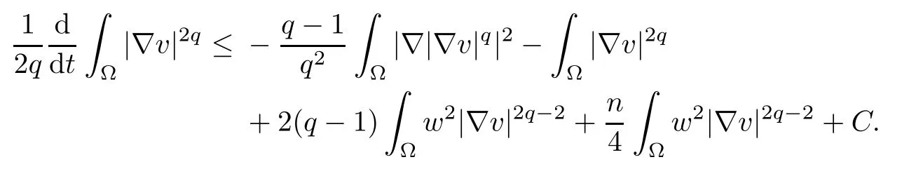
Using Young’s equality once again, we have

and

where θ1and θ2are given by (2.1) and (2.2).

Combining (3.6) with (3.13), we obtain

which implies (3.1).

To cancel the first integral on the right hand of (3.1), we establish a differential inequality involvingby the third equation in (1.1).

Lemma 3.2Let T ∈(0,Tmax), and the assumptions (1.2)–(1.5) hold. Then, there exists C >0 independent of T such that the solution of (1.1) fulfills

ProofTesting the third equation (1.1) by wp+γ?2integrating with respect to x ∈?, we obtain

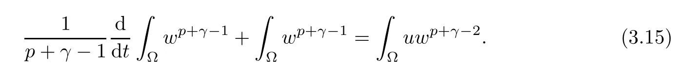
Using Young’s equality, we obtain

This yields (3.14).

The first integral on the right side of (3.1) can be canceled by an appropriate linear combination of (3.1) and (3.14). Thus, we have the following results.

Lemma 3.3Let T ∈(0,Tmax) and the assumptions in Theorem 1 hold. Then, there exists C >0 independent of T such that the solution of (1.1) has the property

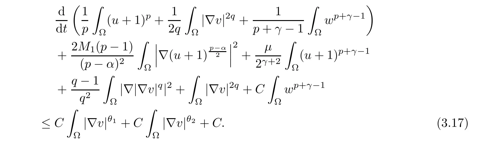
Proofθ1and θ2are given by (2.1) and (2.2). (3.17) results from (3.1) and (3.14) by a simple calculation.

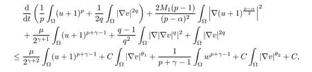
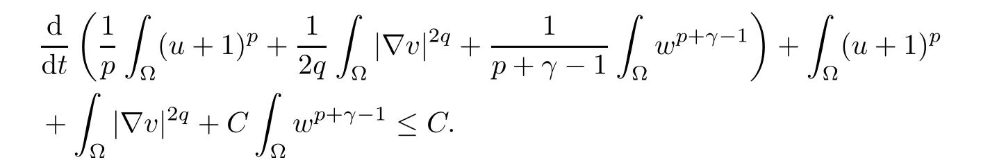
Now, we can obtain a boundedness foraccording to the two integrals on the right hand side of (3.17).

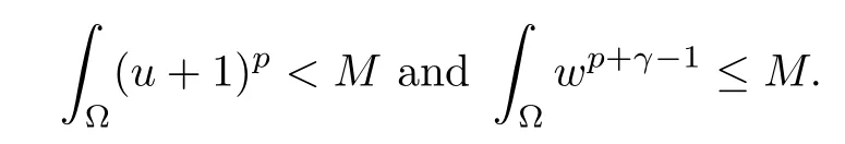
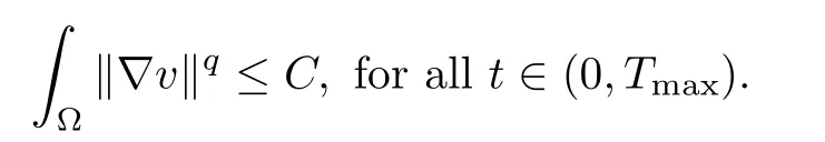
Lemma 3.4Let T ∈(0,Tmax), the assumptions(1.2)–(1.5)hold and

Then, there exists a constant M >0 independent of T such that the solution of (1.1) satisfies

ProofUsing Young’s inequality, we obtain

According to the Gagliardo-Nirenberg inequality, for i=1,2, pick C >0 such that

where kiis defined by (2.3), and the Young’s inequality show that

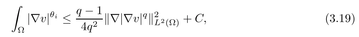
for i=1,2. Then from the above inequality (3.18) and (3.19), we can find a positive constant C >0 such that

Set

The standard ODE comparison theorem implies that

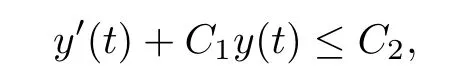
where C1and C2are positive constants.

On the basis of the above lemma, we can obtain the proof of Theorem 1.1.

Proof of Theorem 1.1For any q >2, there exists c(q)>0 such that

Relying on this and the assumptions (1.2)–(1.5), for any p>1, there exists c(p) such that

Now, with the help of the iteration procedure of Alikakos-Moser type [21], we obtain

and then, with the aid of some parabolic regularity theory or ODE theory to the Neumann problem vt=?v+w ?v and wt=u ?w, we obtain

Hence, this completes the proof.