BOUNDEDNESS OF THE FRACTIONAL INTEGRAL OPERATOR WITH ROUGH KERNEL AND ITS COMMUTATOR IN VANISHING GENERALIZED VARIABLE EXPONENT MORREY SPACES ON UNBOUNDED SETS
2020-02-21 01:27:28MOHuixiaWANGXiaojuanHANZhe
數(shù)學(xué)雜志 2020年1期
MO Hui-xia, WANG Xiao-juan, HAN Zhe
(School of Science, Beijing University of Posts and Telecommunications, Beijing 100876, China)
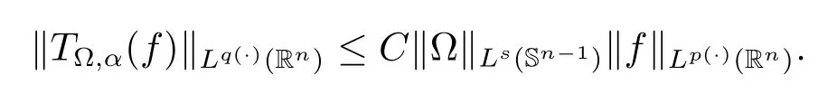
Abstract: In this paper, we study the boundedness of fractional integral operators and their commutators in vanishing generalized Morrey spaces with variable exponent on unbounded sets.Using the properties of variable exponent functions and the pointwise estimates of operators T?,α and their commutators[b,T?,α]in Lebesgue spaces with variable exponent,we obtain the boundedness of fractional integral operators T?,α and their commutators [b,T?,α]in vanishing generalized Morrey spaces with variable exponents on unbounded sets, which extend the previous results.
Keywords: fractional integral operator with rough kernel; commutator; BMO function space; vanishing generalized Morrey space with variable exponents
1 Introduction
In recent years, the theory of variable exponent function spaces attracted ever more attention (see [1–8]for example), since Kovik and Pkosnk [1]introduced the variable exponents Lebesgue and Sobolev spaces, which are the fundamental works of variable exponent function spaces.The function spaces with variable exponent were applied widely in the image processing, fluid mechanics and partial differential equations with non-standard growth (see [9–13]for example).
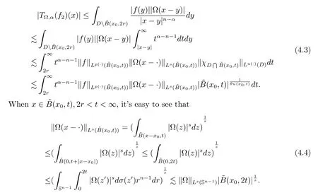
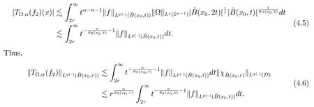
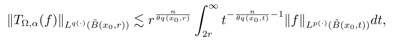
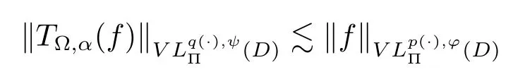
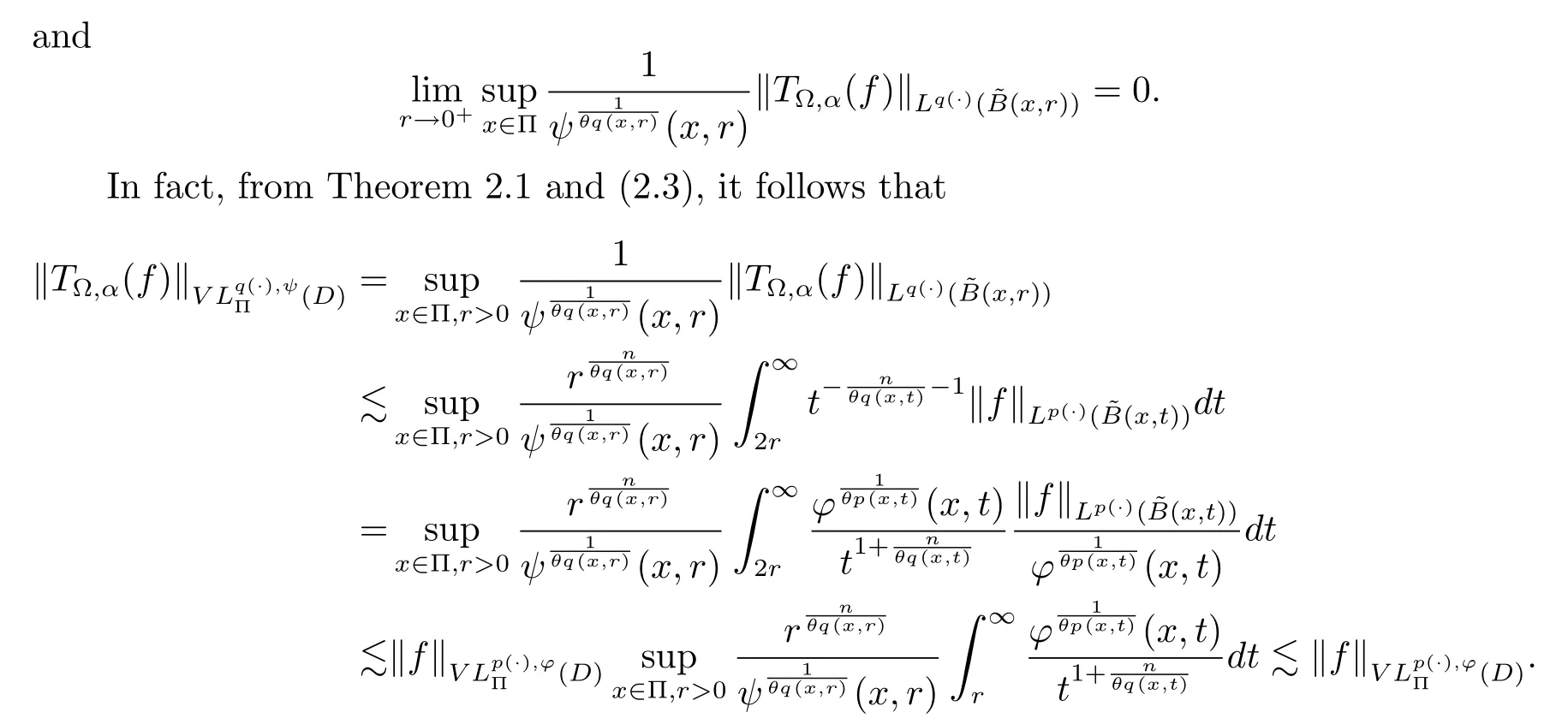
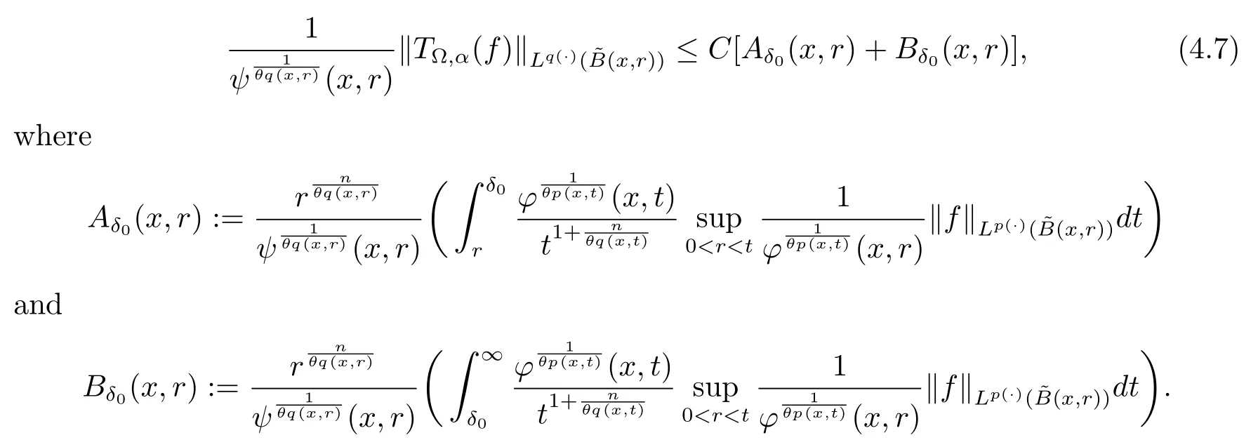
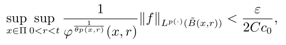
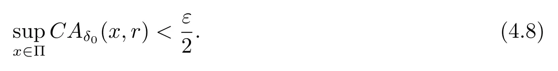
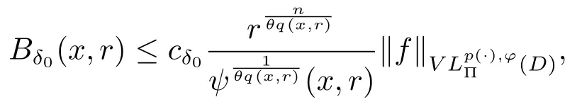
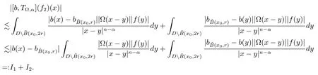
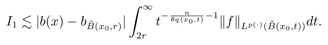
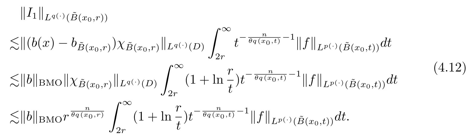
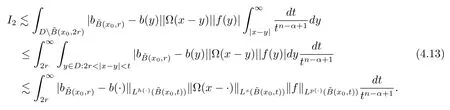
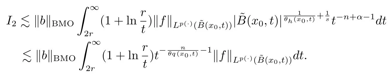
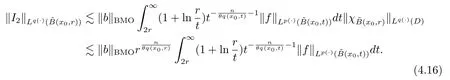
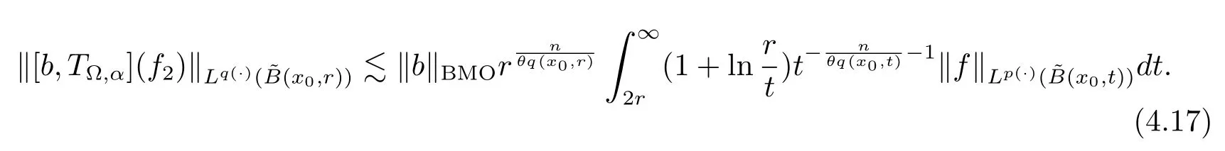
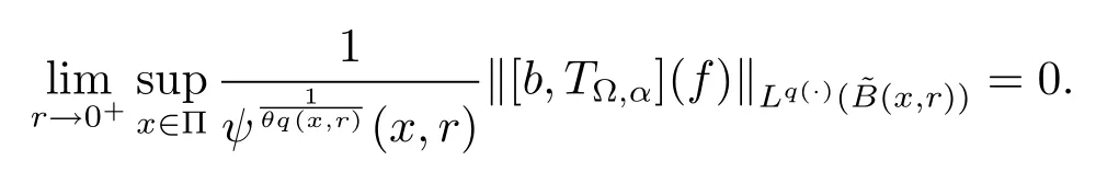
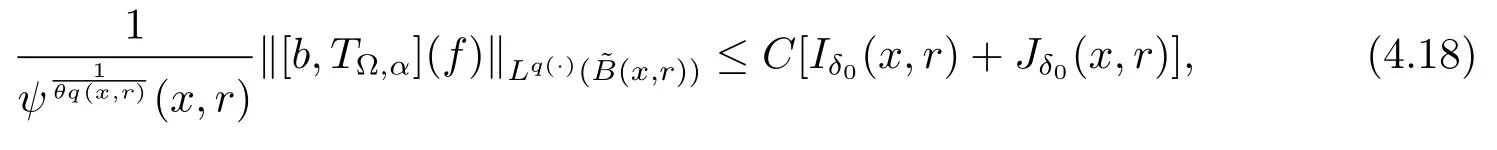
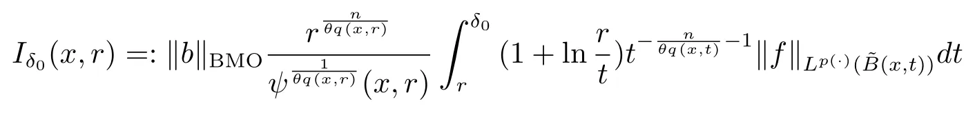
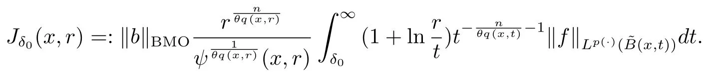
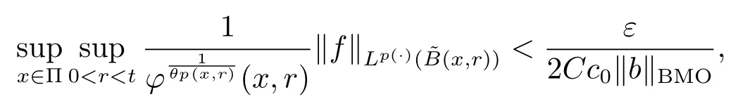
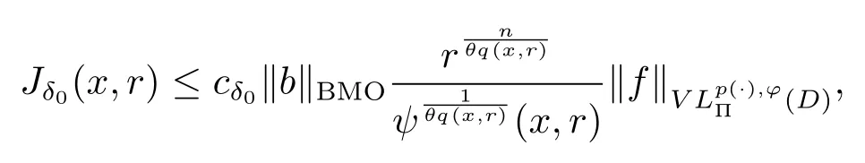
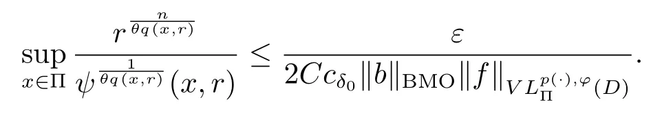
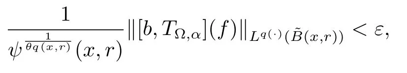
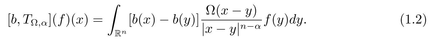
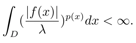
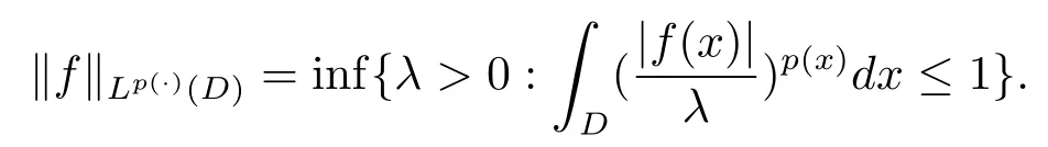
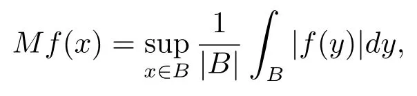
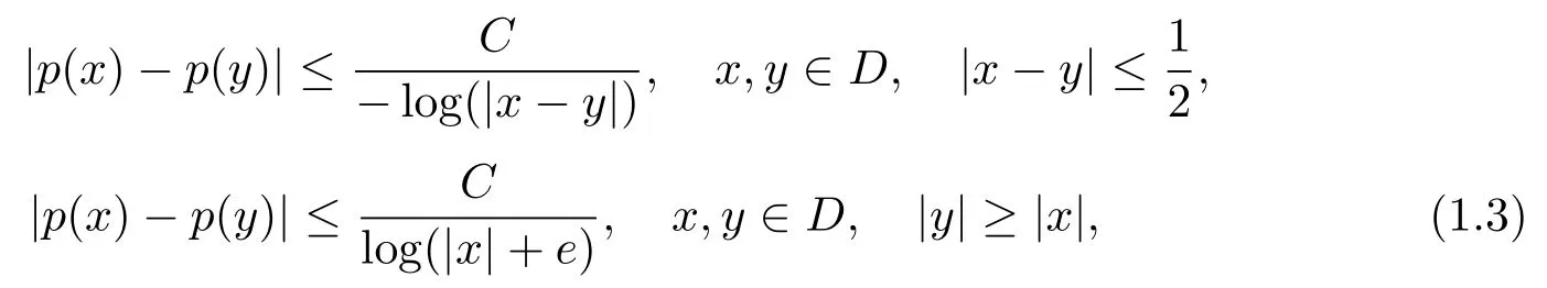
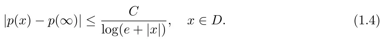
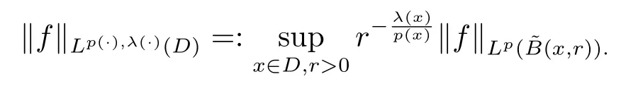
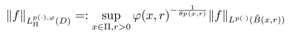
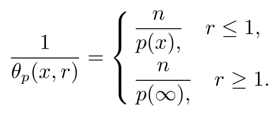
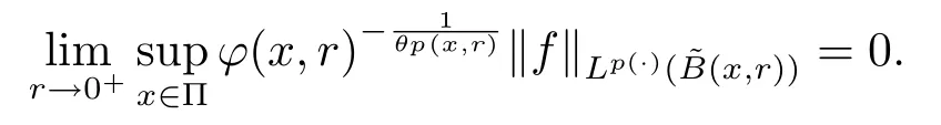
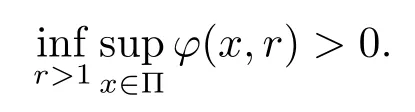
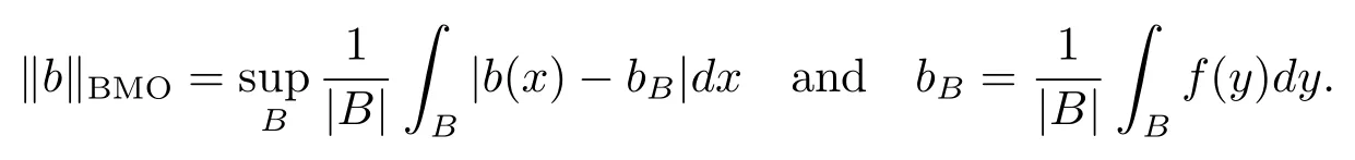
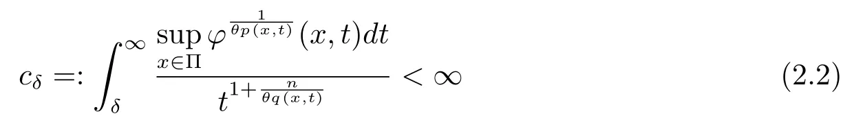
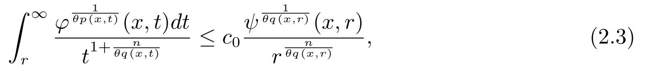
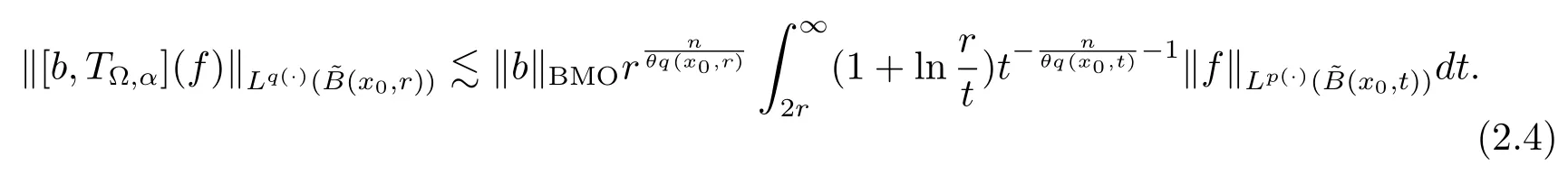
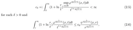
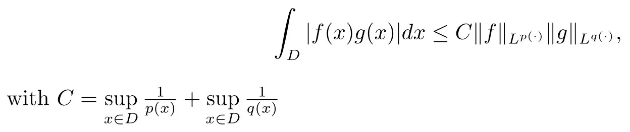
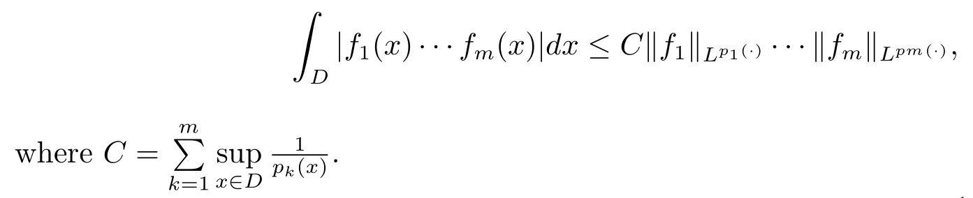
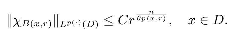
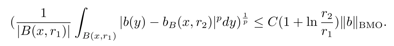
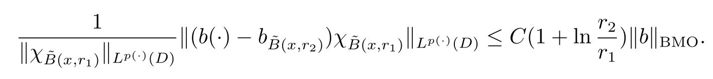
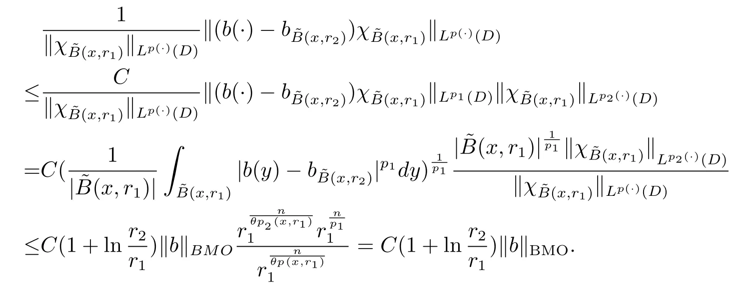
Let ?∈Ls(Sn?1) be homogeneous of degree zero on Rn, where Sn?1denotes the unit sphere of Rn(n ≥2) equipped with the normalized Lebesgue measuredσands ≥1.For 0<α Moreover, letb ∈Then the commutator generated byT?,αandbcan be defined as follows Recently, Tan and Liu [14]studied the boundedness ofT?,αon the variable exponent Lebesgue, Hardy and Herz-type Hardy spaces.Wang [15]et al.obtained the boundedness ofT?,αand its commutator [b,T?,α]on Morrey-Herz space with variable exponent.Tan and Zhao [16]established the boundedness ofT?,αand its commutator [b,T?,α]in variable exponent Morrey spaces.In 2016, Long and Han [17]established the boundedness of the maximal operator, potential operator and singular operator of Calden-Zygmund type in the vanishing generalized Morrey spaces with variable exponent. Inspired by [14–17], in the paper, we consider the boundedness ofT?,αand its commutator [b,T?,α]generated byT?,αand BMO functions in vanishing generalized Morrey spaces with variable exponent on unbounded sets. NotationThroughout this paper, Rnis then-dimensional Euclidean space,χAis the characteristic function of a setA ?Rn;Cis the positive constant, which may have different values even in the same line;ABmeans thatA ≤CBwith some positive constantCindependent of appropriate quantities and ifABandBA, we writeA≈B. Now, let us recall some necessary definitions and notations. Definition 1.1LetD ?Rnbe an open set andp(·) :D →[1,∞) be a measurable function.Then,Lp(·)(D) denotes the set of all measurable functionsfonDsuch that for someλ>0, This set becomes a Banach function space when equipped with the Luxemburg-Nakano norm Lp(·)(D) is regarded as variable exponent Lebesgue space.And, ifp(x)=pis a positive constant, thenLp(·)(D) is exactly the Lebesgue spaceLp(D). Define the setsP0(D) andP(D) as followsP0(D) ={p(·) :D →[0,∞),p?> 0,p+<∞}, andP(D) ={p(·) :D →[1,∞),p?> 1,p+<∞}, wherep?=and Definition 1.2Letf ∈then the Hardy-Littlewood maximal operator is defined by where the supremum is taken over all balls containingx. LetB(D) be the set ofp(·)∈P(D) such that the Hardy-Littlewood maximal operatorMis bounded onLp(·)(D). Definition 1.3[18]LetD ?Rnbe an open setD ?Rnandp(·)∈P(Rn).p(·) is log-Hlder continuous, ifp(·) satisfies the following conditions we denote byp(·)∈Plog(D).From Theorem 1.1 of[18],we know that ifp(·)∈Plog(D),thenp(·)∈B(D). IfDis an unbounded set, we shall also use the assumption: there existsp(∞) =:And, we denote the subset ofwith the exponents satisfying the following decay condition, Note that ifDis an unbounded set andp(∞)exists,then(1.4)is equivalent to condition(1.3).We would also like to remark thatif and only ifand LetD ?Rnbe an open set andwhereB(x,r)is the ball centered atxand with radiusr. Definition 1.4[3] For 0<λ(·) Definition 1.5LetD ?Rnbe an unbounded open set and Π?D,?(x,r) belongs to the classof non-negative functions on Π × [0,∞), which are positive on Π × (0,∞).Then for 1≤p(x)≤p+<∞, the generalized Morrey space with variable exponent is defined by and Definition 1.6LetD ?Rnbe an unbounded open set.The vanishing generalized Morrey space with variable exponentis defined as the space of functionsf ∈such that Naturally, it is suitable to impose on?(x,r) with the following conditions and Noting that, if we replaceθp(x,r) withp(x) in Definition 1.5 and Definition 1.6, thenis the class vanishing generalized Morrey spaces with variable exponent,see[17]for example.Particularly,ifθp(x,r)=p(x),?(x,r)=rλ(x)and Π =D,then the generalized Morrey space with variable exponentis exactly the Morrey space with variable exponentLp(·),λ(·)(D). Definition 1.7Forb ∈then the space of functions of bounded mean oscillation is defined by BMO(Rn)=where In the following, let us state the main results of the paper. Theorem 2.1Assume thatD ?Rnis an unbounded open set.Let 0<α Theorem 2.2Assume thatD ?Rnis an unbounded open set and Π?D.Let 0<α for eachδ>0, and wherec0does not depend onx ∈Π andr>0. Theorem 2.3Assume thatD ?Rnis an unbounded open set.Let 0<α Theorem 2.4Assume thatD ?Rnis an unbounded open set and Π?D.Let 0<α wherec0does not depend onx ∈Π andr>0. In this part, we give some requisite lemmas. Lemma 3.1(see [19, 20])(Generalized Hlder’s inequality) LetD ?Rn,p(·),q(·)∈P(Rn) such thatandg ∈Lq(·)(D), then In general, ifp1(·),p2(·)...pm(·)∈P(Rn) such thatx ∈D.Then forfi ∈Lpi(·)(D),i=1,2,...,m, we have Lemma 3.2(see[21]) LetIfp+ Lemma 3.3(see [5], Corollary 4.5.9) IfDis an unbounded set andthen Lemma 3.4(see [22]) Letb ∈BMO(Rn),1 Lemma 3.5LetD ?Rnbe an unbounded open set,b ∈BMO(Rn)andp(·)Then for anyx ∈D,0 ProofLetsuch thatx ∈D.Then by Lemma 3.2, Lemma 3.3 and Lemma 3.4, we obtain Lemma 3.6(see [23]) Letp(·),q(·)∈P(Rn),0then there existsC>0 such that Lemma 3.7(see[23]) Letb ∈BMO(Rn),p(·),q(·)∈P(Rn),0withthen there exists a constantC>0 such that In this section, we will give the proofs of the main results. Proof of Theorem 2.1Letthen we havef=f1+f2.By the sublinearity of the operatorT?,α, we obtain that For the other part, let us estimate|T?,α(f2)(x)| for Whenx ∈it is easy to see that|x0?y|≈|x ?y|.Letx ∈D.Then by the generalized Hlder’s inequality and Lemma 3.3, we obtain Combining the estimates of (4.1), (4.2) and (4.6) we have which completes the proof of Theorem 2.1. Proof of Theorem 2.2For everywe need to prove that Now, let us show that For 0 For anyε>0, now we choose a fixedδ0such that whenever 0 wherec0andCare constants from (2.3) and (4.7), which is possible since This allows us to estimate the first term uniformly for 0 By choosingrsmall enough, we obtain the estimate of the second term.Indeed, by (2.2),we get wherecδ0is the constant from (2.2).Sinceψsatisfies condition (1.6), we can choosersmall enough such that Combining the estimates of (4.8) and (4.9), we obtain Proof of Theorem 2.3Letthen we havef=f1+f2.Thus, it follows that For the second part of (4.10), let us estimatefirst.It is easy to see that From (4.5), it is easy to see that Thus, according to Lemma 3.3 and Lemma 3.5, we deduce that Whenx ∈B(x0,r) andit is easy to see that|x0?y|≈|x ?y|.Letx ∈D.Then forby Lemma 3.1,we obtain From (4.4) and Lemma 3.5, we have and Thus From (4.12) and (4.16), we get Combining the estimates of(4.10),(4.11)and(4.17),we completed the proof of Theorem 2.3. Proof of Theorem 2.4The proof is similar to that of Theorem 2.2.From Theorem 2.3 and (2.6), it is easy to see thatSo, we just have to show that For 0 where and For anyε>0, now we choose a fixedδ0>0 such that whenever 0 whereandCare constants from (2.6) and (4.18), respectively.It is possible sincef ∈This allows us to estimate the first term uniformly for 0 For the second part, from (2.5), it follows that wherecδ0is the constant from(2.5).Sinceψsatisfies condition(1.6), it is possible to choosersmall enough such that Thus So, from the estimates of (4.19) and (4.20), it follows that which means that Therefore, the proof of Theorem 2.4 is completed.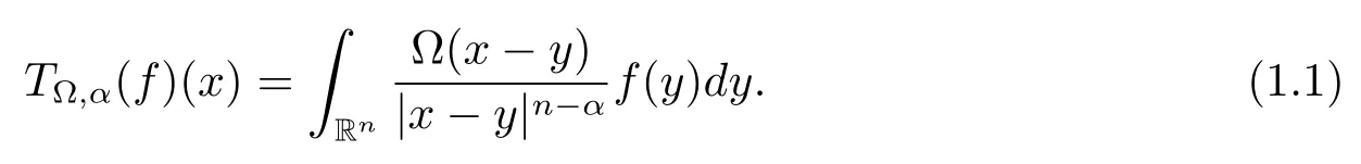

2 Main Results

3 Some Lemmas

4 Proof of Main Results