Peiyuan Fu(符培源), Zhesen Yang(楊哲森),?, and Jiangping Hu(胡江平)

1Beijing National Laboratory for Condensed Matter Physics,and Institute of Physics,Chinese Academy of Sciences,Beijing 100190,China

2School of Physical Sciences,University of Chinese Academy of Sciences,Beijing 100049,China

3Kavli Institute of Theoretical Sciences,University of Chinese Academy of Sciences,Beijing 100190,China

4Collaborative Innovation Center of Quantum Matter,Beijing 100190,China

Keywords: nodal points,chiral symmetry,k·p model

1. Introduction

Topology has emerged as a central concept in the research field of condensed matter physics for over 30 years.[1-3]By combining topology and band theory, we can calculate the Berry connection which can be viewed as a U(1)gauge field in the Brillouin zone (BZ) to obtain a topological quantity,the Chern number. Hence, all the two-dimensional insulators can be further classified by the Chern class,based on the first Chern number. Inspired by this new approach to classify the phase of matter beyond the Landau’s spontaneous symmetry breaking approach, many new states of gapped phases have been found both theoretically and experimentally,such as quantum spin Hall insulators, three-dimensional topological insulators, topological crystalline insulators, and topological superconductors.[4-8]These new phases all focus on gapped systems,whose Berry connection and Berry curvature can be well defined in the whole BZ.

Recently, the concepts of topology are found to be well defined in gapless systems, namely, topological protected semimetals (TS).[9]In these semimetals, there exist topologically stable band degeneracies in the BZ, which are robust against weak (symmetry preserving) perturbations. According to the dimension of band degeneracies, these topological protected semimetals can be classified roughly into the nodal point (NP) and nodal line semimetals. For the former case, the band degeneracies are discrete points in the BZ, such as Weyl semimetals, Dirac semimetals, and type-II Weyl semimetals.[10-12]For the latter case, the band degeneracies are one-dimensional nodal lines in the BZ,which can form loops,chains,links,or even knots.[13-19]Many topological semimetal phases have been predicted by first-principles calculations[20]and observed by angle-resolved photoemission spectroscopy (ARPES) experiments.[21]Searching for new topological phases and possible emergent behaviors has been new research frontiers both theoretically and experimentally.[22-38]

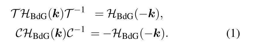
In general, the topologically stable band degeneracies are protected by discrete symmetries and global topological invariants, e.g., Chern number,[1]winding number,[39]or Z2charge.[4,6]The topological stability of band degeneracies means that the NPs or nodal lines cannot be eliminated by symmetry preserving perturbations. In this paper, we consider a two-dimensional multi-band model with chiral symmetry,and study the NPs evolutions under possible small perturbations. The model can be interpreted as a Bogoliubovde Gennes (BdG) Hamiltonian with time-reversal symmetry in addition to the electron band model. Under the time reversal T and the particle-hole symmetry C, a BdG Hamiltonian transfers as[40]

The chiral symmetry S is the combination of T and C as S =T C. By calculating the moving directions of the NPs under generic forms of symmetry preserving perturbations, we classify the local evolutions of nodal points by the type of k·p models around these points.

2. Hamiltonian and symmetry

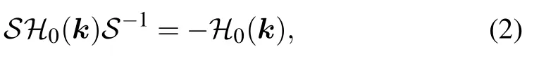
Consider a general multi-band Bloch Hamiltonian H0(k)with chiral symmetry S=σz. Under the chiral symmetry,

from the anti-commutation relations of Pauli matrices{σi,σj}=δij, we can easily check that the Hamiltonian can be written as

where σ±=(σx±iσy)/2. The condition for the band crossing is determined by the vanishing of det[H0(k)],which can be expressed as det[H0(k)]=det[H+0(k)]det[H-0(k)]=0. Since det[H+0(k)]=det[H-0(k)]?, the condition for gap closing is reduced to the following condition:

where γr0(k) and γi0(k) are the real and imaginary parts of det[H+0], respectively. Generally, if we consider a twodimensional(2d)system with k=(kx,ky),the solution of is discrete points(nodal points)in the BZ,as the co-dimension of the degeneracies is 2 = 2-0.[41]These NPs are stable against chiral symmetry preserving weak perturbations. Now assuming there exists a nodal point NP0at k0=(k0,x,k0,y)in the BZ,we ask how will this NP moves under perturbations.

In general,a chiral symmetry preserving perturbation can be written as

where λ is the external parameter to control the perturbation,H=H0+H1. When λ →0,H →H0. Under this perturbation,the gap closing condition is determined by

Obviously,γr/i(k,λ)satisfies γr/i(k,λ =0)=γr/i0 (k). Hence we can re-express the equations for the gap closing under perturbations as=-This expression simplifies the discussion in the next section.

3. Nodal points evolutions

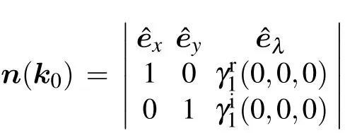
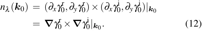
Now we want to track the motion of the NP0in the BZ as λ changes. Without loss of generality, we can assume λ ＞0 in the following discussion. We consider a 2-band model for simplicity, which can be generalized to multi-band cases using the method we discuss below. The observation is that we can regard λ as a third dimension in addition to the original 2d BZ. Thus the band degeneracies of the Hamiltonian H0(k)+H1(k,λ)are 1d nodal lines which contain NP0,namely, k0, as shown in Fig. 1. The NP0moves along the tangential direction of the nodal line under perturbations. Notice that the nodal line lies on both surfaces γr/i(k,λ)=0,as shown in Fig.1. So its tangent vector n(k0,λ =0)is perpendicular to the gradient directions nr(k0,λ =0)=?γr(k0,0)and ni(k0,λ =0)=?γi(k0,0)of these two surfaces,respectively, as shown in Figs. 1(a) and 1(b). We write them down explicitly for further convenience

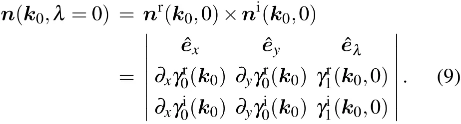
Notice that n(k0,λ =0) can also be defined as ni(k0,0)×nr(k0,0), which means we have two directions. However,only one of them is the moving direction with λ ＞0. We clarify that the moving direction is determined by the third component of n(k0,0),which is

If nλ(k0,0)＞0, the moving direction of NP0is the projection of n(k0,0)in the λ =0 plan(which is the 2d BZ of the original Hamiltonian H0(k)),(nx(k0,0),ny(k0,0)),as shown in Fig.1(d). If nλ(k0,0)＜0,the moving direction of the NP is (-nx(k0,0),-ny(k0,0)). Next we use some concrete examples to illustrate the above procedures and provide some insight into the classification of the local evolutions.

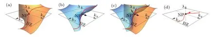
Fig.1.The method to determine the moving direction of a NP(black dot at the original point).Panels(a)and(b)show the surfaces γr0+λγr1=0,γi0+λγi1=0 and their normal directions,respectively. Panel(c)shows that the tangential direction of the NL(with red color)is perpendicular to the above two normal directions. (d)The projection of the NL onto the λ =0 plan is the trajectory of the NP and the tangential direction is the moving direction.

4. Examples

In the first example, we take γr0= sinkx, γi0= sinky,γr1=1+sinky,and γr1=λ+2sinkx.

The band degeneracies occur at(0,0),(π,0),(0,π),and(π,π) in the 1st Brillouin zone. As they are locally separated, we can only consider the NP at k0= (0,0) for simplicity, which is shown in Fig. 2(a1). Around this point, the k·p model can be written as γr0?kx,γi0?ky,γr1?1+ky,and γi1?λ+2kx. After a simple calculation, we obtain the two normal directions nx(k0) = (1,0,1) and nz(k0) = (0,1,0).Based on these results, we can obtain the moving direction n(k0)=(-1,0,1),as shown in Fig.2(a2). Because nλ(k0)＞0,this NP moves along the-?exdirection under the perturbation with 1 ?λ ＞0, as shown in Fig.2(a3). The NP moves along this direction, and cannot be eliminated by small external perturbations, as shown in Fig. 2(a4). This feature is only determined by the property of k·p Hamiltonian at the NP. Indeed, if we add a more general kind of perturbation H1(kx,ky,λ) = λγr1(kx,ky,λ)σx+λγi1(kx,ky,λ)σz, the moving direction n(k0)is

Thus the moving direction of the NP in the BZ k0is(-γr1(0,0,0),-γi1(0,0,0)). We can easily check that the NP just moves in the BZ and cannot disappear or transit to multi-NPs unless γr1(0,0,0)=γi1(0,0,0)=0 under small finite perturbations.

In the second example,we take γr0=1-coskx,γi0=sinky,γr1=1+sinky,and γi1=λ+2sinkx.

In this case,we choose the NP at(0,0),the effective k·p Hamiltonian around the NP is γr0?k2x/2,γi0?ky,γr1?1+ky,and γi1?λ+2kx, as shown in Fig. 2(b1). Thus the two normal directions are nx(k0) = (0,0,1) and nz(k0) = (0,1,0)and the moving direction is n(k0)=(-1,0,0), as shown in Fig. 2(b2). However, there is a crucial difference compared to example 1, that is, the third component of n(k0) is zero,which is nλ(k0)=0 and n(k0)/=0. Note that the NL is either above or blow the λ =0 plan. We can check that external perturbations either eliminate the NP or transit it into two NPs.Figure 2(b4)shows the transition to two NPs with a finite perturbation 0 ＞λ ?-1. Notice that this feature is related to the band dispersion around the NP in which the dispersions are linear along one direction and quadratic along the other.

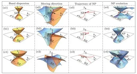
Fig.2. The classification of the evolutions of nodal points. The classification is based on the first column,that is nλ(k0)and n(k0). The second and third columns show the constraints of the band dispersion around the NP and the possible geometry forms of the nodal line in kx-ky-λ space passing the NP, respectively. The last column shows the possible evolutions of NPs under a general form of perturbations. One can notice that the Dirac point(with linear dispersion along every direction)is stable against any chiral symmetric perturbation and cannot disappear nor transit to multi-NPs.

In the third example, we take γr0=1-coskx, γi0=1-cosky,γr1=1+sinky,and γi1=3+λ+2sinkx.

In this case,the effective k·p Hamiltonian around the NP(0,0)is γr0?k2x/2,γi0?k2y/2,γr1?1+ky,and γi1?3+λ+2kx,as shown in Fig. 2(c1). Thus the two normal directions are nx(k0)=(0,0,1)and nz(k0)=(0,0,3)and the moving direction is n(k0)=(0,0,0),as shown in Fig.2(c2).Notice that the calculated n(k0)is equal to zero,which means the nodal line does not have a well defined tangential direction at this point as shown in Fig.2(c3).The external perturbations either eliminate the NP or transit it into multi-NPs.Figure 2(b4)shows the transition to four NPs with a finite perturbation 0 ＞λ ?-1.Notice that this feature is related to the band dispersion around the NP,which is non-linear along all directions.

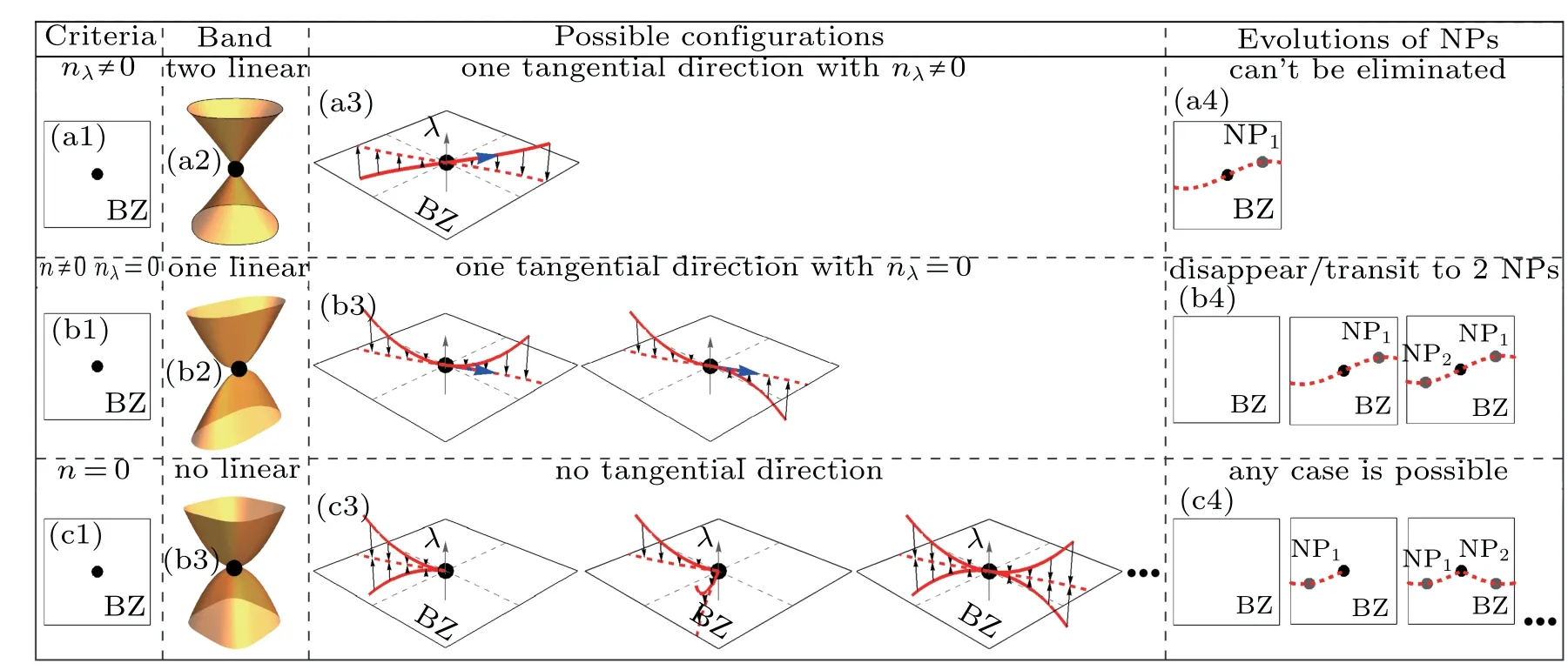
Fig. 3. The classification of the evolutions of nodal points. The classification is based on the first column, that is nλ(k0) and n(k0). The second and third columns show the constraints of the band dispersion around the NP and the possible geometry forms of the nodal line in kx-ky-λ space passing the NP,respectively. The last column shows the possible evolutions of NPs under a general form of perturbations. One can notice that the Dirac point (with linear dispersion along every direction) is stable against any chiral symmetric perturbation and cannot disappear nor transit to multi-NPs.

These different features of the NP evolutions under perturbations reveal that NPs may have inner structures. We discuss these findings in detail in the following.

5. Classification of the evolutions

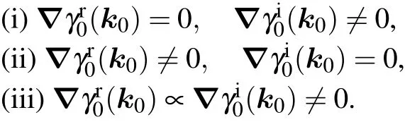
According to the above examples, we can classify the evolutions of the NPs by the third component of the moving direction n(k0)into three cases

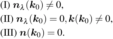
We first notice that the above three classes are complete.Any 2d kind of NP must belong to one of them. The next step is to find the constraints of the above conditions to the band structure and possible evolutions of NPs. We analyze the three cases respectively.

Case(I)In this case,we first notice

If this term does not equal to zero,one can always take a rotation of the momentum space around the NP k0,such that

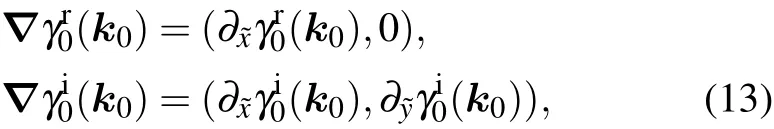
where ??x=?/??kxand ??y=?/??ky. Thus we can write down the effective Hamiltonian around the k0point,which is

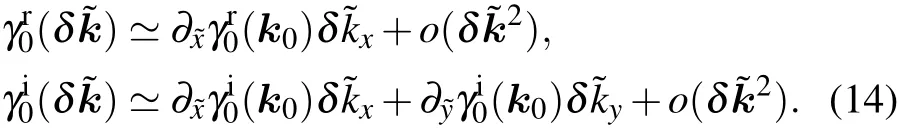
Thus the constraint nλ(k0)/=0 guarantees that the k·p Hamiltonian is linear along every direction around the NP to the leading order. Now we discuss the possible evolutions of NPs.As pointed out before,the evolution of NP depends on the tangential direction of the NL in the kx-ky-λ space. Now if we consider the presence of the tangential direction n(k0) with nλ(k0)/=0 of the NL, the moving direction of the NP in the 2d BZ is

which means the topology of the NL around the NP must be equivalent to that in Fig. 3(a3). And the moving direction of the NP with small perturbations is unique. This kind of NP cannot be eliminated by external perturbations, as shown in Fig.3(a4). The results are summarized in Fig.3(a).

Case(II)The first condition nλ(k0)=0 implies the flowing three possible realizations:

The effective k·p Hamiltonian under these constrains can be written down as

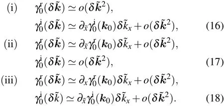
These mean the dispersions at the NP are linear in one direction and quadratic or higher orders in the other to the leading order.

The second equation n(k0)/=0 requires the perturbation satisfying

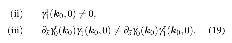
The conditions nλ(k0)=0 and n(k0)/=0 require that the tangential direction of the NL at the NP is in the λ =0 plan and the possible topology of the NL around the NP is shown in in Fig.3(b3). Any external perturbation satisfying Eq.(19)transits it into two NPs or disappears. This case is summarized in Fig.3(b).

Case (III) In this case, we first emphasize that we classify the general kind of perturbation terms. In case (II), if the perturbation terms break Eq.(19), the NP with linear and quadratic dispersions also satisfies n(k0)=0. However, this requires a special kind of perturbation. Thus we do not consider this case in our classification tables. A more general case satisfying n(k0)=0 is

This means the k·p Hamiltonian around the NP has quadratic or higher order dispersion to the leading order along both directions. The vanishing of n(k0) implies that the NP is a singularity point on the NL. The results are summarized in Fig.3(c).

6. Conclusion

We study the evolutions of NPs in systems with chiral symmetry, which can host discrete nodal points in the BZ.Figure 3 shows the classification of the NP evolutions under general form of perturbations. We exhaust all the possible evolution types of NPs and show that the classification can be achieved according to the type of k·p model around the NPs.Only the nodal points with linear dispersion along every direction are robust against perturbations and cannot be gapped.