Shanshan GUO(郭閃閃)

School of Mathematical Sciences,Xiamen University,Xiamen 361005,China E-mail:guoshanshan0516@163.com

Zhong TAN(譚忠)?

School of Mathematical Sciences and Fujian Provincial Key Laboratory on Mathematical Modeling and Scienti fic Computing,Xiamen University,Xiamen 361005,China E-mail:tan85@xmu.edu.cn

Abstract This work consider boundary integrability of the weak solutions of a non-Newtonian compressible fluids in a bounded domain in dimension three,which has the constitutive equations as

Key words compressible fluid;weak solutions;non-Newtonian fluids;integrability

1 Introduction

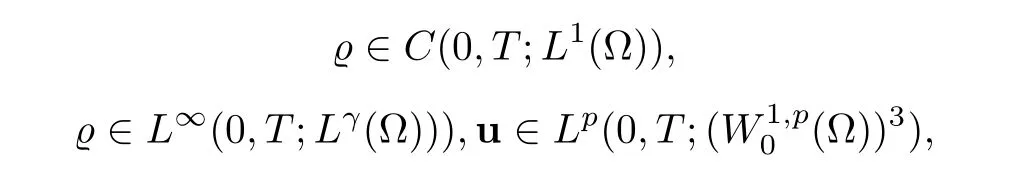
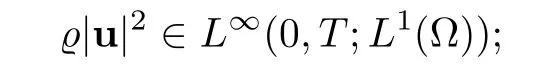
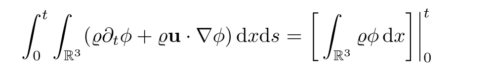
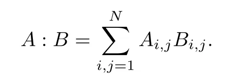
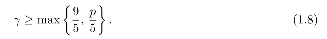
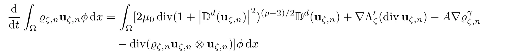
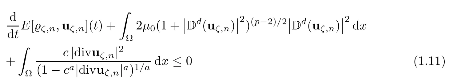
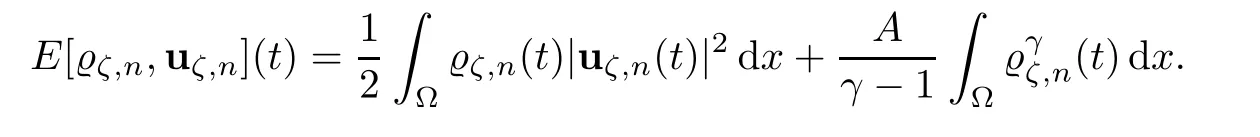
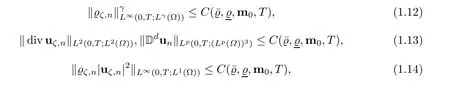
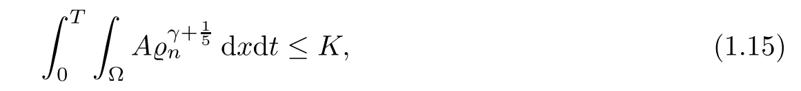
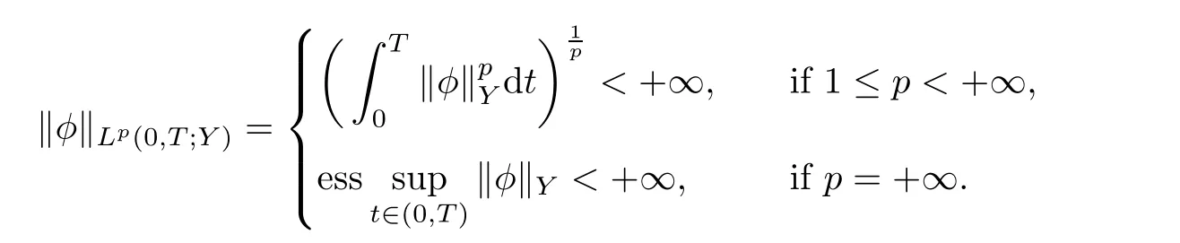
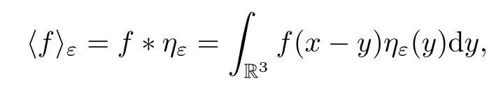
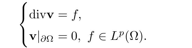
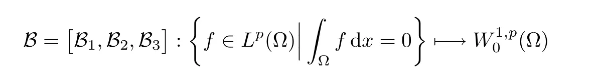
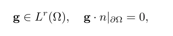
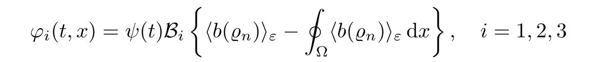
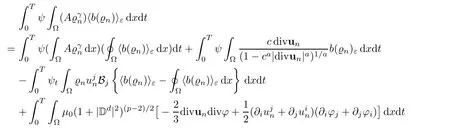
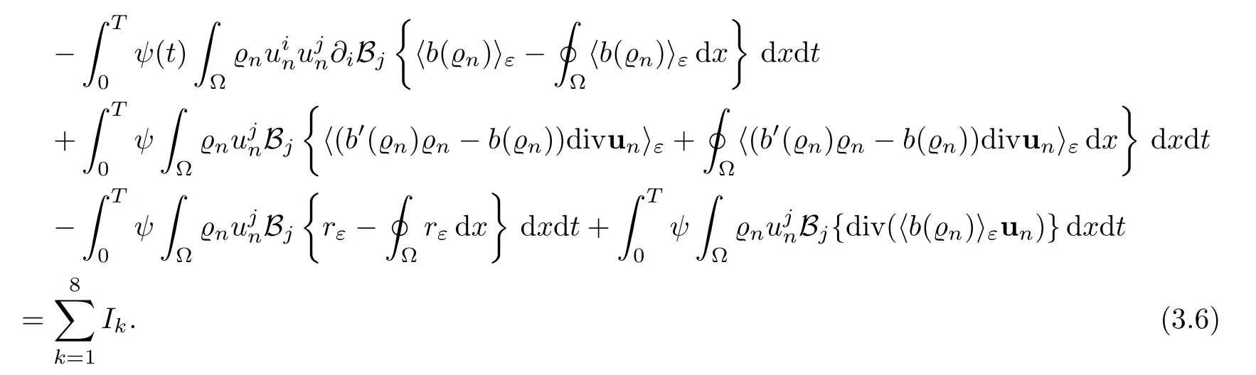
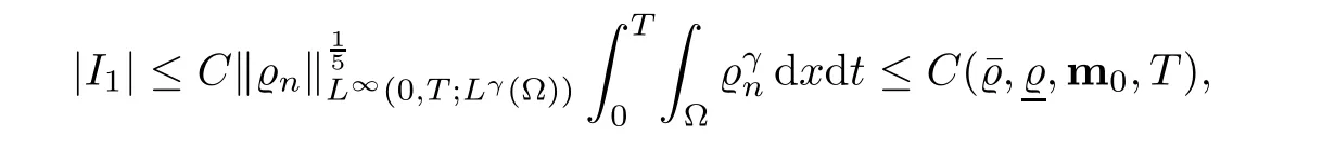
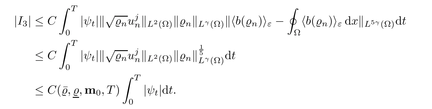
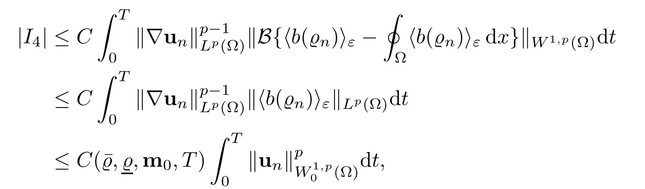
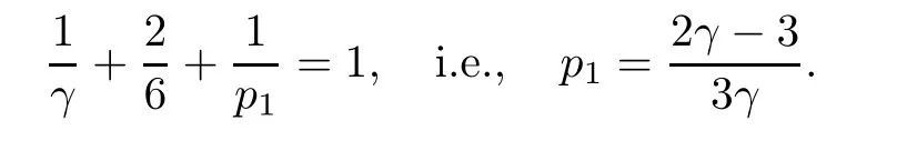
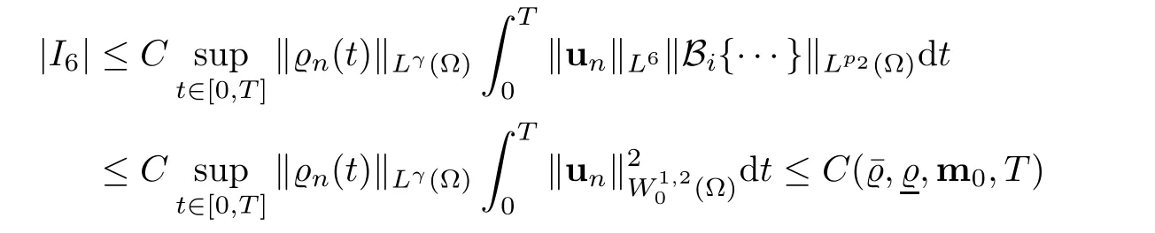
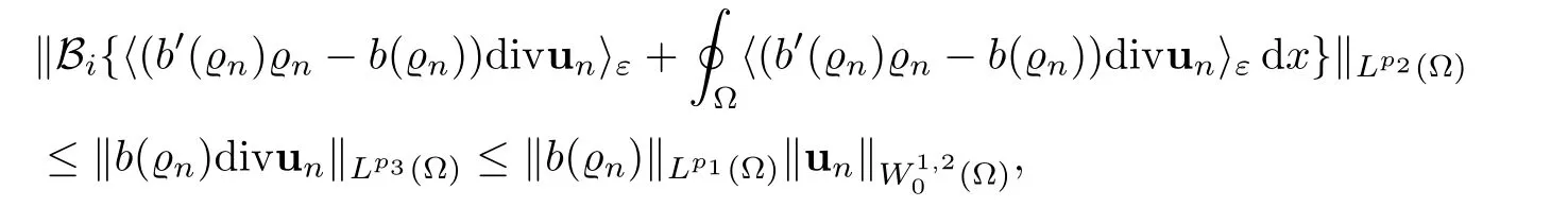
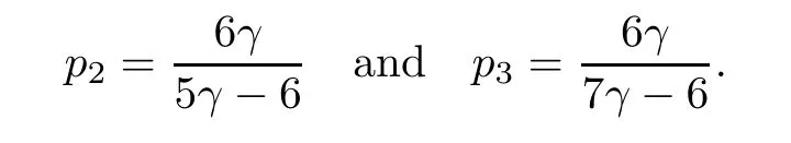
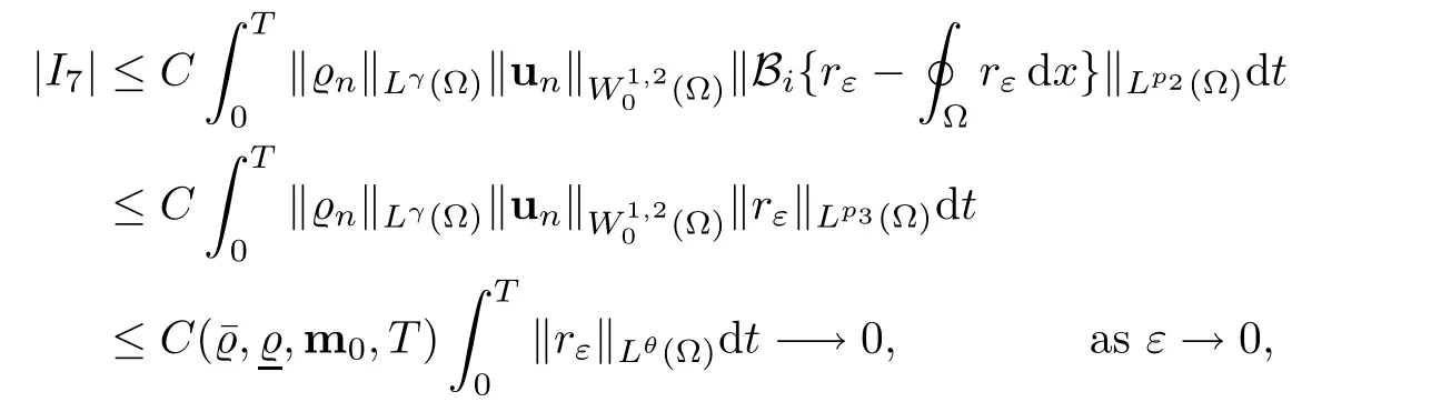
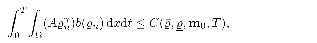
Let ? ? R3be a bounded domain with Lipschitz boundary,for 0

with

where t∈ (0,T)is time,x∈ ? is the spatial coordinate,=(t,x)∈ (0,∞)is the density function,u(t,x)=(u1,u2,u3)represents the velocity of the fluid.P():=Aγstands for the scalar pressure,μ0,a,c and A are positive constant,γ >1 is the adiabatic constant,p∈[11/5,∞).The symbolstands for Cauchy stress tensor,denotes the symmetric gradient of the velocity u,we also use Ddfor the traceless part of D,that isI is the 3×3 identical matrix,the symbol?stands for the tensor product,u?u={uiuj}.

Initial-boundary value conditions.We assume the no-slip boundary condition

At the initial time,we assume

Notice that,for the constitutive equations of non-Newtonian fluids,the relation between the stress S and the strain rate is nonlinear.Otherwise,if the relation is linear,the fluid is called Newtonian,in this case,we have the classical Navier-Stokes equations,which have the enormous amount of e ff orts[1–7],and so on.The main characteristics of a non-Newtonian behavior are the ability of the fluids to shear thinning or shear thickening in shear flow,the presence of non-zero normal stress di ff erences in shear flow,the ability of the fluids to yield stress and the ability of the fluids to creep.For an introduction to the mechanics of non-Newtonian fluids,one can refer to[8,9].

For non-Newtonian fluids,the first results on existence and uniqueness of weak solutions were achieved by Ladyzhenskaya in[5]and by Lions in[10]forbased on monotone operators and compactness arguments.For the incompressible cases,Diening-R?u?i?ka-Wolf[11]showed the existence of fluids of power-law type based on Lipschitz truncation method forin all dimension n ≥ 2.Using the setting of implicit constitutive relations,Bulí?ek et al.[12]established long-time and large-data of weak solutions for three-dimensional bodies with the Navier slip boundary conditions.We also refer to[13–15,21],and references therein.

Based on Galerkin approximation,Feireisl et al.[16]showed that there exists a weak solution(,u)to a class of non-Newtonian compressible fluids with the scalar pressure P=P()satis fied

In this work,we consider the system(1.1)–(1.6)with a nonlinear pressure equation P()=Aγ,just like[16],with minor modi fications,we can get that there exists a weak solution(,u)to the system(1.1)–(1.6).Inspired by the work of Feireisl and Petzeltová[17],we want to show that the density is square integrable up to the boundary with the help of the linear operator B.Similarly as[16],the de finition of weak solutions to the problem(1.1)–(1.6)is listed as follow.

De finition 1.1The weak solution of the problem(1.1)–(1.6)is a pair of functions(,u)such that

(1)

(2)the equation of continuity(1.1)holds in the sense of distributions on(0,T)×R3

Remark1.The special nonlinear constitutive equations(1.3)guarantees the boundedness of divu,which means|divu|<.Based on this,the authors in[16]introduced a convex potential Λ :R → [0,∞],

2.Here the symbol A:B stands for the scalar product

Theorem 1.2Let T>0,the adiabatic constant γ satisfy

is said to be a weak solution of(1.1)–(1.6),especially,we have

In the spirit of[18,Chapter 6],we first replace Λ by a smooth regularization function λζ,use Galerkin method to find an approximation solution(ζ,n,uζ,n)of the problem(1.1)–(1.6)with the initial data

By applying fixed point theorem,we can show that,for any T>0,given u∈C([0,T],Xm),there exist a unique solution=[u]solves equation(1.1),and the map u →[u]is continuous.Consequently,we may find an approximation solution(uζ,n,ζ,n)of the integral equation

for all φ ∈ Xm,whereζ,n=[uζ,n].Especially,take φ =uζ,n,we have the following energy inequality

in D′(0,T),where

The energy inequality(1.11)gives rise to the following estimates

where constants C are independent of n and ζ.

To prove Theorem 1.2,we need to establish the following assertion first,which is also the core of this paper.For simplicity of notation,we shall write(n,un)instead of(ζ,n,uζ,n).

Theorem 1.3A function pair(n,un),which is the approximation solution of the system(1.1)–(1.6)with initial data(1.10),satis fies the following inequality

where K is a constant,independent of n.

Just like[16],the limit of the approximation(n,un)is the weak solutions of original problems(1.1)–(1.6),thus,passage to the limit in(1.15)yields the conclusion of Theorem 1.2.Therefore,in the rest part,our main work is to proof Theorem 1.3.

Let us introduce some notations and function spaces,which will be used in the sequence of this article.

Notations1.Let 1≤p≤∞,k∈N.Bywe denote the usual Sobolev space.Let(Y,k·kY)be a normed space.By Lp(0,T;Y),we denote the space of all Bochner measurable functions φ :(0,T)→ Y such that

2.The symbol C denotes a generic positive constant,which may vary in di ff erent estimates.

3.Let hfiεrepresent the molli fier of f,satisfying

where ηεdenotes the Friedrichs’molli fier.

2 A Bounded Linear Operator B

In this section,we recall some properties for operators constructed by Bogovskii[19]in order to help us obtain the crucial inequality(1.15)in Theorem 1.3.In other words,these operators are solutions to the problem

Lemma 2.1Let ??R3be a bounded domain with Lipschitz boundary.It can be shown that there exists an operator B enjoying the properties

(1)

is a bounded linear operator,i.e.,

for any 1

(2)The function v=B{f}solves the problem

(3)Moreover,if f can be written in the form f=divg for a certain

then

for arbitrarily 1

ProofOne can refer to Gladi[1,Theroem 3.3]or Bochers and Sohr[20,Theorem 2.4]for the detail proof. ?

3 Proof of Theorem 1.3

Let us begin with some auxiliary lemmas.

Lemma 3.1(see[6,Lemma 2.3]) Let ? ? Rnbe a domain,u ∈ W1,α(?),∈ Lβ(?),1≤α,β≤∞.For K ??? (if ?=Rn,K can be Rn),we have

Furthermore,we have following lemma.

Lemma 3.2Prolongingnand unby zero outside ?,we have

holds in D′((0,T)×R3)for any b∈ C1(R),globally Lipschitz on R.

ProofThe proof of(3.1)can be found in[17,Lemma 3.1].Regularizing equation(3.1)and using Lemma 3.1,one can deduce(3.2). ?

RemarkFurthermore,by virtue of(3.2),we have the following assertion

where

using Lemma 3.1(ii),

Next,we will give the proof of Theorem 1.3.

Proof Theorem 1.3Consider the quantities

as test functions for(1.2),where 0≤ψ≤1,ψ∈D(T,T+1),and

Combining Lemmas 2.1,3.1 and 3.2,by straightforward computation,we have

Here and in what follows,we use the summation convention to simplify notation.In the following,we consider the estimates of the eight integrals.

(i)Using(1.12),we have

where the constant C is independently of n and ε.

(ii)By the help of the H?lder inequality,(1.12)and(1.13),we get

(iii)Combining the Sobolev embedding inequality and(2.1),we obtain

(iv)The integral I4may be estimated as follows

last equality holds by the reason of

(v)For the term I5,by virtue of the H?lder inequality and(2.1),we find that

where

Making use of hypothesis(1.8),one gets

which implies

Combining(1.12)and(1.13),we ascertain,I5is bounded independently of n,ε as above.

(vi)The integral I6can be controlled by

with the fact that

where

(vii)Furthermore,we get

last inequality is obtained by the help of(3.5),(3.4)and(3.7).

(viii)Similarly as the integral I6,making use of(2.3),we conclude

Summing the previous estimates(i)–(viii)and letting ψ → 1, ε→ 0,making use of the Fatou’s lemma,we have

independently of n.Thus,we get(1.15).Hence,we conclude the proof. ?