
LARGE TIME BEHAVIOR OF SOLUTION TO NONLINEAR DIRAC EQUATION IN 1+1 DIMENSIONS?
2019-05-31 03:39:20YongqianZHANG張永前
Yongqian ZHANG(張永前)
School of Mathematical Sciences,Fudan University,Shanghai 200433,China E-mail:yongqianz@fudan.edu.cn
Qin ZHAO(趙勤)?
School of Mathematical Sciences,Shanghai Jiao Tong University,Shanghai 200240,China E-mail:zhao@sjtu.edu.cn
Abstract This paper studies the large time behavior of solution for a class of nonlinear massless Dirac equations in R1+1.It is shown that the solution will tend to travelling wave solution when time tends to in finity.
Key words large time behavior;nonlinear Dirac equation;gross-Neveu model;global strong solution;gravelling wave solution
1 Introduction
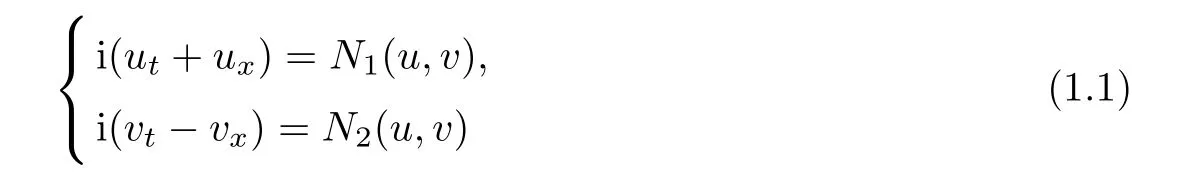
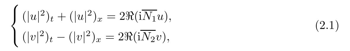
We are concerned with the large time behavior of solution for the nonlinear Dirac equations
with initial data

where(t,x)∈R2,(u,v)∈C2.The nonlinear terms take the following form

with
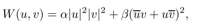
where α,β ∈ R1andare complex conjugate of u and v.(1.1)is called Thirring equation for α =1 and β =0,while it is called Gross-Neveu equation for α =0 and β =1/4;see for instance[9,14,18].
There were many works devoted to study the Cauchy problem for nonlinear Dirac equations,see for example[2–4,6–8,10,11,14,15,17,19]and the references therein.The survey of wellposedness and stability results for nonlinear Dirac equations in one dimension was given in[14].Recently,the global existence of solutions in L2for Thirring model in R1+1was established by Candy in[4],while the well-posedness for solutions with low regularity for Gross-Neveu model in R1+1was obtained in Huh and Moon[12],and in Zhang and Zhao[20].
Our aim is to establish the large time behaviour of solution to(1.1)and(1.2).Similar to[1],it is shown that the solution will tend to travelling wave solution when time tends to in finity.The main results are stated as follows.
Theorem 1.1For any solution(u,v)∈ C([0,∞),Hs(R1))with,there hold that,

and

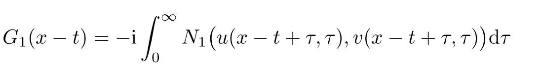
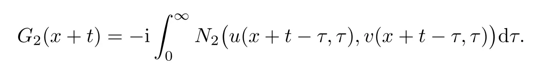
where
and
Moreover,we have
and
Theorem 1.2For any strong solution(u,v)∈ C([0,∞),L2(R1)),there exists a pair of functions(g1,g2)∈L2(R1)such that

and

Here the strong solution to(1.1)and(1.2)is de fined in following sense.
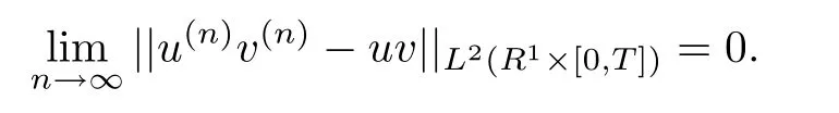
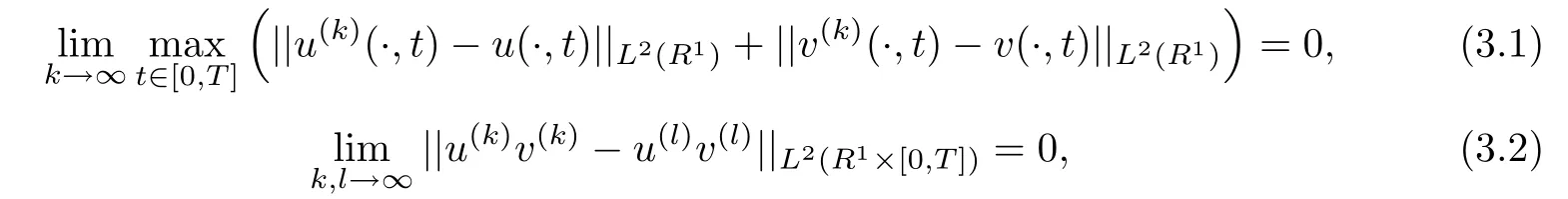
De finition 1.3A pair of functions(u,v)∈ C([0,∞);L2(R1))is called a strong solution to(1.1)and(1.2)on R1× [0,∞)if there exits a sequence of classical solutions(u(n),v(n))to(1.1)on R1×[0,∞)such that

and
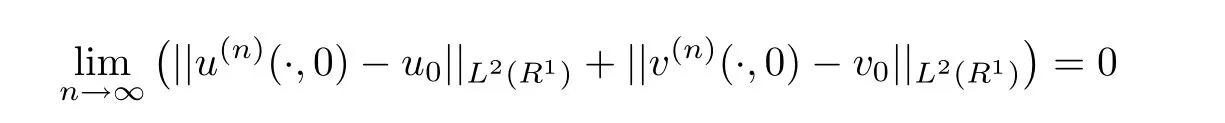
for any T>0.
Remark 1.4The strong solution was de fined for the linear hyperbolic equations,see for instance,[5,13,16].Here we de fine the strong solution for nonlinear dirac equations in the same way as in[16].
Remark 1.5For any sequence of classical solutions(u(n),v(n))given as in De finition 1.3,it was shown in[20]that for any T>0,there holds the following,
Therefore,the strong solution(u,v)is also a weak solution to(1.1)and(1.2)in distribution sense.
The remaining of the paper is organized as follows.In Section 2 we first recall Huh’s result on the global well-posedness in C([0,∞);Hs(R1))for s>1/2 for(1.1).Then we use the characteristic method to establish asymptotic estimates on the global classical solutions and prove Theorem 1.1.In Section 3 we prove Theorem 1.2 for the case of strong solution.
2 Asymptotic Estimates on the Global Classical Solutions
The global existence of the solution into(1.1)and(1.2)forwas obtained by Huh in[11].We consider the smooth solution(u,v)∈ C1(R1×[0,∞))to(1.1)and(1.2)in this section.
Multiplying the first equation of(1.1)by u and the second equation by v gives
which,together with the structure of nonlinear terms,leads to the following,

Now we consider the solution(u,v)in the triangle domain.For any a,b∈R1with a

see Figure 1.
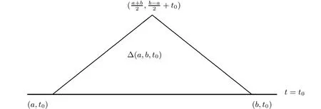
Figure 1 Domain?(a,b,t0)
It is obvious that?(a,b,t0)is bounded by two characteristic lines and t=t0.The vertices ofare(a,t0),(b,t0)and
Lemma 2.1For anythere holds that
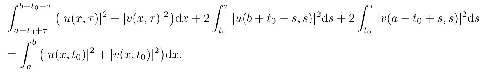
ProofAs in Huh[11],we can get the result by taking the integration of(2.2)over the domain

The proof is completed.
A special example of Lemma 2.1 is the following estimate on the domain?(x0?t0,x0+t0,0)for any x0∈R1and t0>0,

With above lemma,we can derive the following pointwise estimates on the triangle via the characteristic method.
Lemma 2.2Suppose thatfor some constant C0>0.Then there hold that
and

for x∈R1,t≥0.
Remark 2.3We remark that estimates(2.4)and(2.5)in Lemma 2.2 were proved by Huh in[11]for R1×[0,∞)and we give the sketch of the proof here.Indeed,(2.1)gives
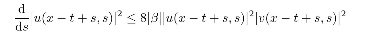
and

Then,taking the integration of the above from 0 to t yields that
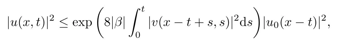
which implies estimate(2.4)on u by(2.3).Estimate(2.5)on v could be derived in the same way.
Lemma 2.4There exists a constant C>0,such that for any t≥0,there hold the following
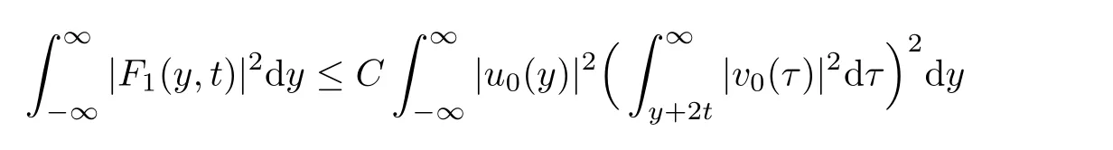
and
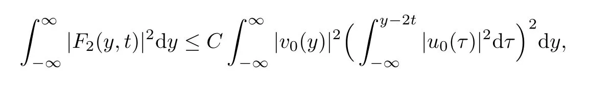
where
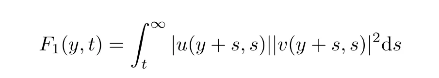
and
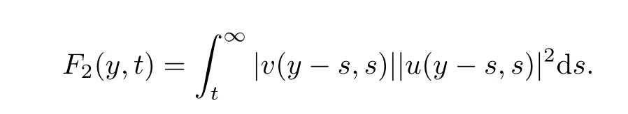
ProofBy Lemma 2.2,we have
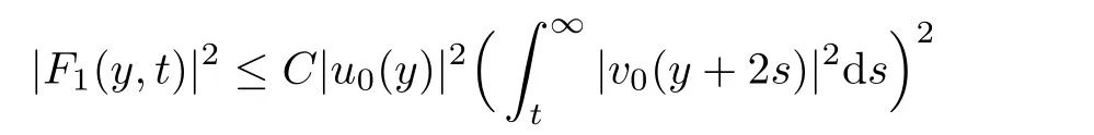
for some constant C>0.Then
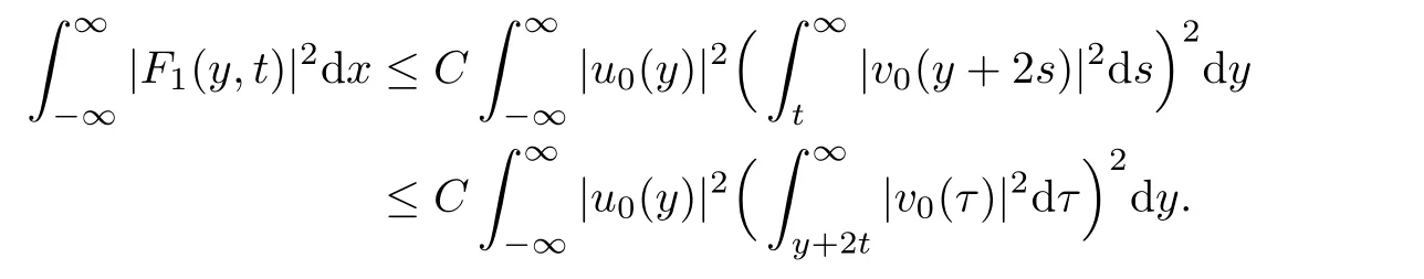
The inequality for F2could be proved in the same way.The proof is completed.
Lemma 2.5There hold that

and
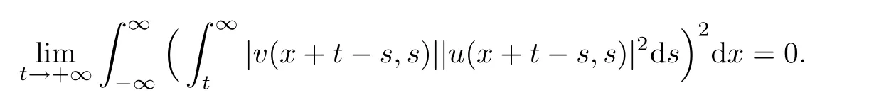
ProofBy Lemma 2.4,we have
Since
then the first inequality follows by Lebesgue’s dominant convergence theorem.The second inequality could be proved in the same way.The proof is completed.
Before proving Theorem 1.1,let us state the following lemma.
Lemma 2.6For(u0,v0)∈Hs(R1)withthen it holds that
ProofIn fact,we have
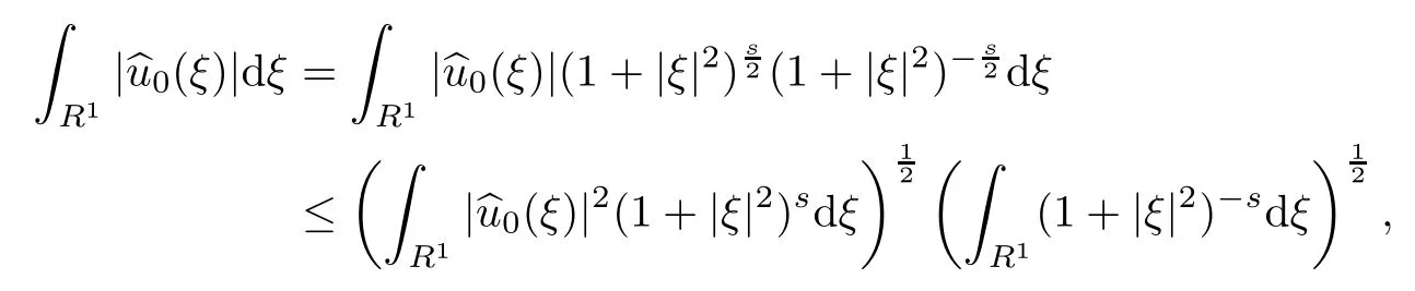
where
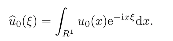

and
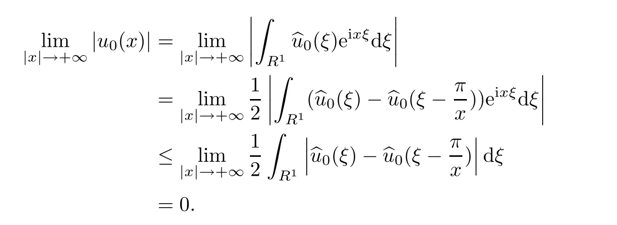
The result on v0could be proved in the same way.The proof is completed.
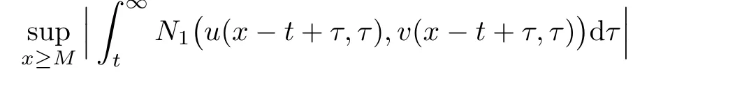
Proof of Theorem 1.1First we use the characteristic method to derive the following

where G1(x?t)is given by Theorem 1.1,and

for some constant C?>0.
Then the asymptotic estimate(1.4)for u follows by Lemma 2.5,and estimate(1.5)for v could be derived in the same way.
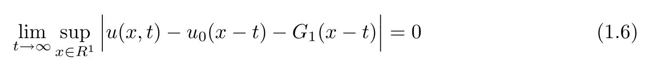
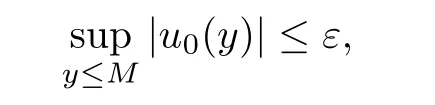
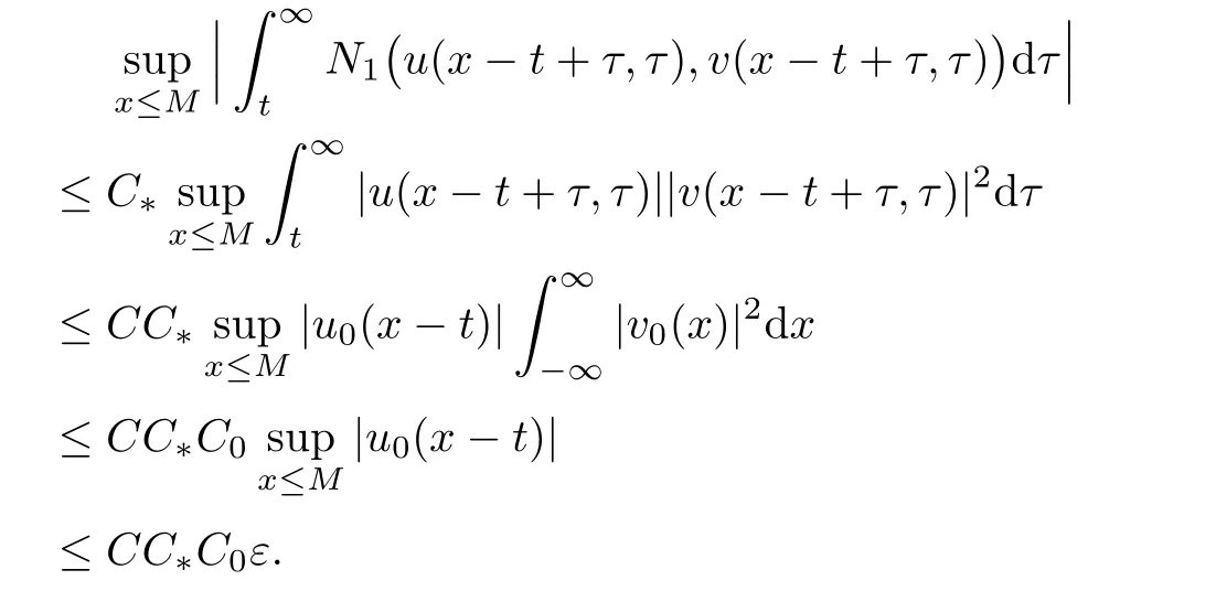
Now to prove(1.6)and(1.7),we need to estimate the remainder term in(2.6)in L∞.We first use Lemma 2.6 to derive that for any ε>0,there is a constant M<0,depending on ε and a constant C>0 such that
which,together with Lemma 2.2,leads to the following
On the other hand,we can obtain
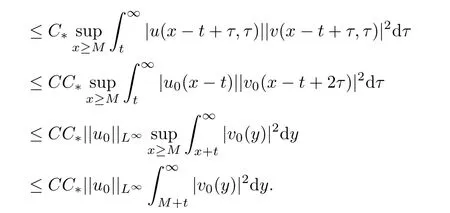
Therefore,with the above estimates,we have

for any ε>0,which yields
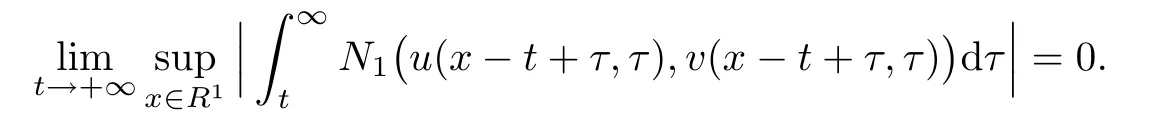
Then it holds that
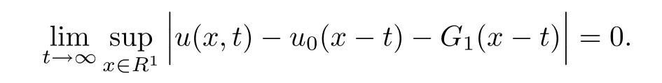
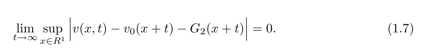
Estimate(1.7)on v could be proved in the same way.The proof is completed.
3 The Case of Strong Solution
Due to[20],for the strong solution(u,v)∈ C([0,∞),L2(R1)),there is a sequence of smooth solutions,(u(k),v(k))of(1.1),satisfying the following
and

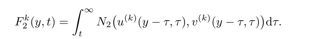
Lemma 3.1For j=1,2,there hold that
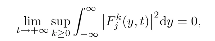
where
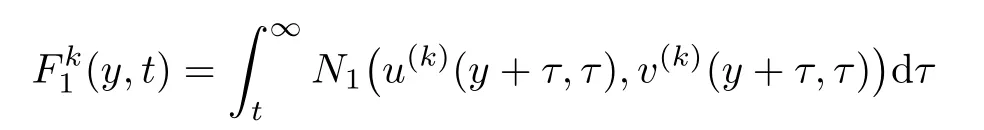
and
ProofLetBy(3.1),we have

Then by Lemma 2.4,we can obtain

Together with(3.1)and(3.4),it implies that for any ε>0,there exists a constant K>0 such that
Therefore,we have
which yields the convergence result for.The convergence forcould be proved in the same way.The proof is completed.
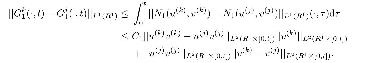
Direct computation gives the following.
Lemma 3.2For any k and j,there exists a constant C1>0 such that

and

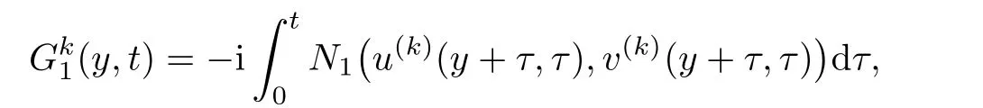
De fine
and
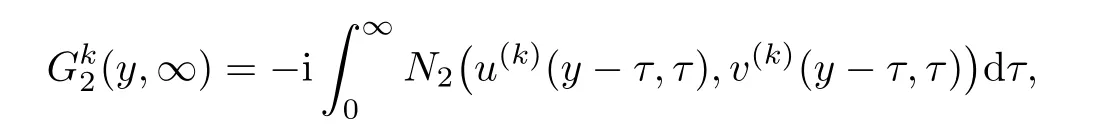
then we have the following lemma.
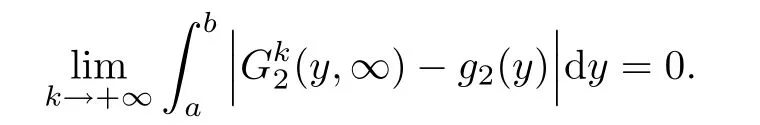
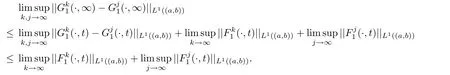
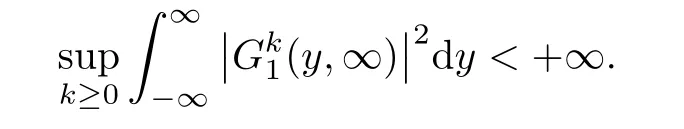
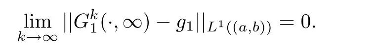
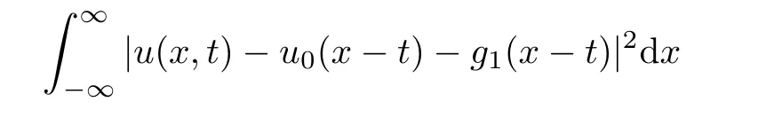
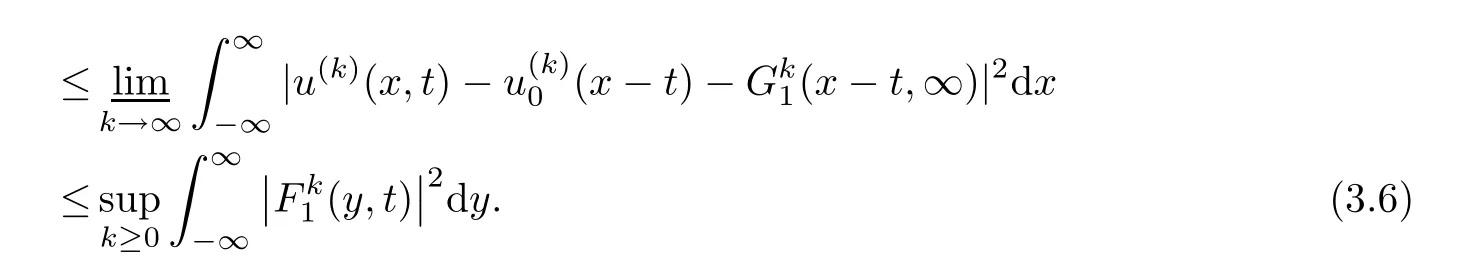
Lemma 3.3There exists a pair of functions(g1,g2)∈L2(R1)such that for any a,b∈R1with a and Moreover,the sequences of functionsandconverge weakly to g1(y)and g2(y),respectively,in L2(R1). ProofLet then by Lemma 3.2,for any t<∞,we can obtain Then,from(3.1)–(3.3),it follows that Therefore,for any a,b∈R1with a Taking t→∞in last inequality,it follows from Lemma 3.1 that On the other hand,by Lemma 3.1,we have Then we can find a function g1∈ L2(R1)such that the sequence of functionsconverges weakly to g1(y)in L2(R1),and Proof of Theorem 1.2We use the notations in the proof of Lemma 3.1 and Lemma 3.3. For smooth solutions(u(k),v(k)),we have which yields Then when k→+∞,by(3.1)and Lemma 3.3,we get the following weak convergence in L2, in L2(R1). Therefore,by the lower semicontinuity of L2-norm with respect to weak topology in L2,see for example[13],we can obtain Let t→+∞,by Lemma 3.1,we can prove(1.8).(1.9)could be proved in the same way.The proof is completed. ?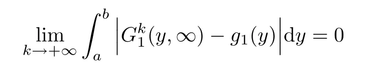


 Acta Mathematica Scientia(English Series)2019年2期