-, -

(Department of Mathematics and Physics, Henan University of Urban Construction, Pingdingshan 467000, China)

Empirical Likelihood Statistical Inference for Partially Linear Model with Restricted Condition

LIUChang-sheng*,LIYong-xian

(DepartmentofMathematicsandPhysics,HenanUniversityofUrbanConstruction,Pingdingshan467000,China)

Inthispaper,weapplytheempiricallikelihoodmethodtopartiallylinearmodelwithparameterlinearrestrictedhypothesis.Forthesakeoftestinghypothesis,anempiricallog-likelihoodratioteststatisticbasedonthedifferenceofthenullandalternativehypothesesisconstructed.Furthermore,thelimitingdistributionoftheteststatisticsisprovedtobeastandardChi-squareddistribution.Numericalsimulationconfirmstheadvantageoftheproposedmethod.

empiricallikelihood;restrictedcondition;partiallylinearmodel;hypothesistest;Chi-squaredistribution

1 Empirical likelihood estimation on parameter

For the need of constructing the test statistic, we first develop estimating approach for model (1) under the null hypothesis in this section. That is, we estimate the unknown quantities in model (1) with the restricted condition Aβ=b.Thenmodel(1)canbewrittenas

(3)

whereKh(·) =K(·/h)/h,K(·) is a kernel function andh=hnis a sequence of positive numbers tending to zero, called bandwidth. Simple calculation yields that

(4)

For 1≤i≤n, let

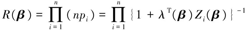
In order to construct the empirical likelihood ratio function, we now introduce one auxiliary random vectorZi(β),

(5)

1.1 Empirical likelihood estimation on parameter without restriction

Next we discuss profile empirical likelihood estimation without restriction conditionsAβ=b. Whenβis true parameter,E(Zi(β))=0. Thus, by the idea of Owen[1], an empirical likelihood-ratio forβcan similarly be defined as follows:

(6)

wherep=(p1,…,pn) is a probability vector.

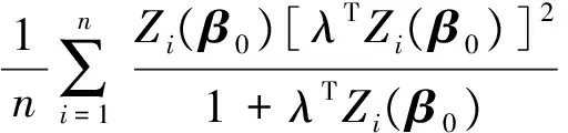
Ifβis true parameter, a unique maximum forpin (6) exists. By the Lagrange multiplier method, the supremum occurs at

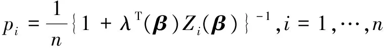
(7)

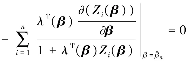
whereλ(β) is the solution to

(8)

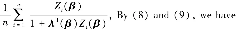
By (6) and (7), we can get

(9)

In the following, we define the profile empirical likelihood estimator without any restriction conditions

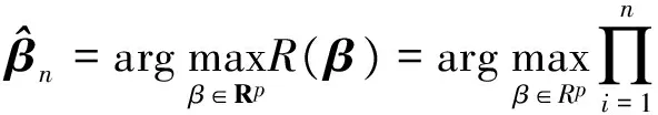
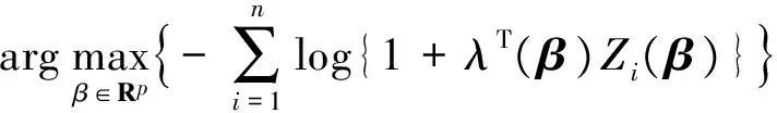
(10)

whereZi(β) andλ(β) satisfy (5) and (8), respectively.

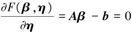
1.2 Empirical likelihood estimation on parameter with restrictionAβ=b

(11)

whereηis ak×1 vector that contains the Lagrange multipliers. By differentiating functionF(β,η) with respect toβandη, we obtain the following equations:

(12)

and

(13)

2 Test statistic and its properties

In order to formulate the main results, we need the following assumptions. These assumptions are quite mild and can be easily satisfied.

Lethj(Ti)=E(Xij|Ti),Vi=Xi-E(Xi|Ti), 1≤i≤n, 1≤j≤p.

Assumption1 E(e|X,T)=0andE(|e|4|X,T)<∞.

Assumption3 g(·)andhj(·)areofoneorderLipschitzcontinuousfunctions.

Assumption 5 The kernel functionK(·) is a bounded symmetric density function with compact support and satisfies ∫K(u)du=1,∫uK(u)du=0 and ∫u2K(u)du<∞.

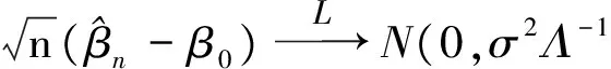
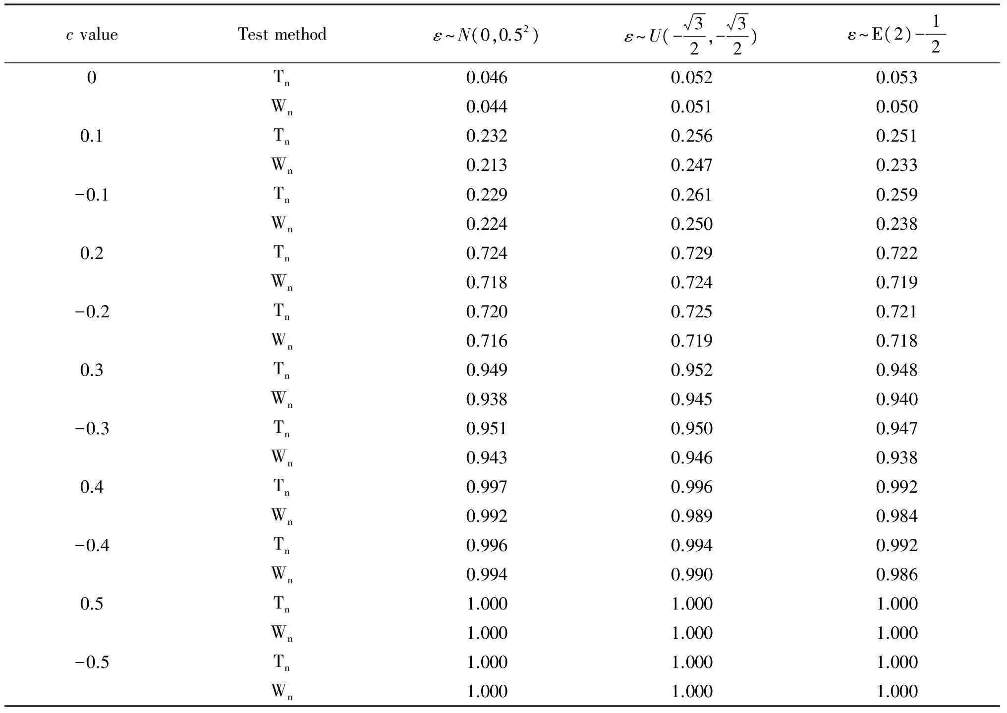
Assumption 6 The density functionsf(t) ofTis bounded away from zero and have bounded continuous second partial derivatives. Namely, 0

Under the above assumptions, we can get the following result, proved in Section 4.

Theorem3Underthenullhypothesisoftestingproblem(1.2)andtheassumptions1-6,wehave

3 Simulation studies

In this section, we present the result of some simulations to illustrate our methods. In our simulations, the data are generated from the following model:

yi=xi1β1+xi2β2+g(ti)+εi,i=1,…,n,

(14)

Tab.1 The rejection frequencies for H0:β1-β2=0?H1:β1-β1=c with α=0.05

We summarize our findings as follows. When the null hypothesis is true (that is,c=0), the rejection frequencies (estimated sizes) of both our proposed test basedTnand the restricted least-squares approach test basedWnare quite good and close to their nominal levels 0.05 under different error distributions. Under the alternative hypothesis, the rejection rate seems very robust to the variation of the type of error distribution. With the increasing ofc, the test power of our proposed test is slightly better than the test based on the residual sum of squares.

4 Proof of the main results

In the sequel, letCdenote positive constant whose value may vary at each occurrence.

Lemma 1 Suppose that Assumptions 1-6 hold.

whereG0(·)=g(·) andGl(·)=hl(·)(j=1,…,p).

ProofTheproofissimilartoLemmaA.1inLiang[9]etal.

Lemma2SupposethatAssumptions1-6hold.Wecanobtain

ProofTheproofissimilartoLemmaA.2inLiang[9]etal.

Lemma3SupposethatAssumptions1-6hold.ifβ0istruevalueofβ, We can obtain

ProofFromthedefinitionofZi(β), we have

Lemma4SupposethatAssumptions1-6hold.Ifβ0istruevalueofβ,Wehavemax1≤i≤n‖Zi(β0)‖=op(n1/2).

ProofAsimilarproofcanbefoundinLiang[10]etal.

Lemma5SupposethatAssumptions1-6hold.Ifβ0isthetruevalueofβinmodel(3),satisfying(7)and(8),thenwehave

ProofApplyingtheTaylorexpansion,from(8)andLemma1～4,weobtainthat

(15)

In view of Lemma 1～4, we have

This completes the proof.

TheproofofTheorem1

(16)

(17)

(18)

where

(19)

We can also get

(20)

This completes the proof.

TheproofofTheorem2issimilarasthatofTheorem1andthusisleftforthereaders.

TheproofofTheorem3

ProofBy(10)andapplyingtheTaylorexpansion,wehave

(21)

where

Similarly, we can also get

(22)

with |r2n|=op(1).

From (21) and (22), we can get

I1+I2+op(1).

Op(n-1)·Op(n1/2)·op(n1/2)=op(1).

(23)

[1]OWENAB.Empiricallikelihoodratioconfidenceintervalsforasinglefunctional[J].Biometrika,1988,75(2):237-249.

[2]OWENAB.Empiricallikelihoodratioconfidenceregions[J].AnnStat, 1990,18(1):90-120.

[3]SHIJ,LAUTS.Empiricallikelihoodforpartiallylinearmodels[J].JMultivAnal, 2000,72(1):132-148.

[4]WANGQH,JINGBY.Empiricallikelihoodforpartiallinearmodelswithfixeddesigns[J].StatProbLett, 1999,41(4):425-433.

[5]WANGQH,JINGBY.Empiricallikelihoodforpartiallylinearmodels[J].AnnInstStatMath, 2003,55(3):585-595.

[6]FANJ.Locallinearregressionsmoothersandtheirminimaxefficiencies[J].AnnStat, 1993,21(1):196-216.

[7]FANJ,GIJBELSI.Localpolynomialmodellinganditsapplications[M].NewTork:Chapman&HallPress, 1996.

[8]WEIC,WANGQ.Statisticalinferenceonrestrictedpartiallylinearadditiveerrors-in-variablesmodels[J].Test, 2012,21(4):757-774.

[9]LIANGH,HRDLEW,CARROLLRJ.Estimationinasemiparametricpartiallylinearerrors-in-variablesmodel[J].AnnStat, 1999,27(5):1519-1535.

[10] LIANG H, THURSTON S W, RUPPERT D,etal. Additive partial linear models with measurement errors[J].Biometrika, 2008,95(3):667-678.

[11] LIANG H Y, JING B Y. Asymptotic normality in partial linear models based on dependent errors[J].J Stat Plan Infer, 2009,139(4):1357-1371.

[12] 洪圣巖. 一類半?yún)?shù)回歸模型的估計理論[J]. 中國科學(xué):A 輯, 1991,34(12):1258-1272.

[13] 孫耀東. 分歧泊松自回歸模型的馬爾可夫性[J]. 湖南師范大學(xué)自然科學(xué)學(xué)報, 2011,34(4):18-20.

[14] WU C. Some algorithmic aspects of the empirical likelihood method in survey sampling[J]. Stat Sin, 2004,14(4):1057-1068.

[15] XUE L G, ZHU L X. Empirical likelihood for a varying coefficient model with longitudinal data[J]. J Am Stat Assoc, 2007,102(478):642-654.

[16] ZHU L, XUE L. Empirical likelihood confidence regions in a partially linear single-index model[J].J Royal Stat Soc: Ser B, 2006,68(3):549-570.

(編輯 HWJ)

2016-03-27

河南省科技計劃項目資助(112300410191)

O

A

1000-2537(2017)04-0075-08

具有限制條件的部分線性模型的經(jīng)驗似然推斷

劉常勝*,李永獻(xiàn)

(河南城建學(xué)院數(shù)理系, 中國 平頂山 467000)

本文將經(jīng)驗似然方法應(yīng)用到具有限制假設(shè)條件的部分線性模型中. 為了檢驗假設(shè)條件, 構(gòu)造基于零假設(shè)和對立假設(shè)條件下的極大經(jīng)驗對數(shù)似然比估計值的差值統(tǒng)計量. 而且在零假設(shè)下證明該統(tǒng)計量的極限分布為標(biāo)準(zhǔn)的χ2分布. 數(shù)值模擬表明所提出的檢驗統(tǒng)計量的優(yōu)勢.

經(jīng)驗似然; 限制條件; 部分線性模型; 假設(shè)檢驗; χ2分布

10.7612/j.issn.1000-2537.2017.04.013

*通訊作者,E-mail：csliu@hncj.edu.cn