Dumitru Baleanu,Jihad H.Asad,and Ivo Petras

1Department of Chemical and Materials Engineering,Faculty of Engineering,King Abdulaziz University,P.O.Box 80204,Jeddah 21589,Saudi Arabia

2Department of Mathematics and Computer Science,Faculty of Arts and Sciences,Cankaya University,06530 Ankara,Turkey

3Institute of Space Sciences,P.O.Box,MG-23,76900,Magurele,Bucharest,Romania

4Department of Physics,College of Arts and Sciences,Palestine Technical University,P.O.Box 7,Tulkarm,Palestine

5BERG Faculty,Technical University of Kosice,B.Nemcovej 3,04200 Kosice,Slovakia

1 Introduction

One of the new directions in fractional calculus and its applications is to investigate the numerical solutions of fractional Euler-Lagrange and Hamiltonian equations.[1?7]These types of equations are new and they involved both left and right derivatives(see for more details Refs.[8–11]and the references therein).

The fractional Hamiltonians are non-local and they are associated with dissipative systems.We recall that Bateman suggested the time-dependent Hamiltonian to describe the dissipative systems.[12]Also,we mention the fact that the time dependent Hamiltonian describing the damped oscillation was introduced by Caldirola[13](see for more details Refs.[14]and[15]).Bateman suggested a variational principle for equations of motion containing a friction linear term in velocity.[12]After more than half century it was f i nd out that the frictional models can be treated naturally within the fractional calculus,[1?6]which studies derivatives and integrals of non-integer order.Constructing a complete description for non-conservative systems can be considered as one of promising applications of fractional calculus.The results reported in Refs.[16–17]are considered as the beginning of the fractional calculus of variations with a deep impact for non-conservative and dissipative processes.Besides,in Ref.[8]it was investigated a Lagrangian formulation for variation problems with both the right and the left fractional derivatives within Riemann–Liouville sense as well as the Lagrangian and Hamiltonian fractional sequential mechanics.

Recently,the numerical methods are used intensively and successfully to solve the fractional nonlinear diあerential equations fractional calculus.[4]

We have used the decomposition method to study the fractional Euler–Lagrange equations for some important three diあerent physical systems,[11,18?20]and we have obtained a numerical solution for the corresponding equations.In two of these references[18?19]we considered the Lagrangian of a Harmonic oscillators,where in Ref.[18]the considered model(i.e.,Pais–Uhlenbeck oscillator)is interesting by itself and in connection with gravity since it involves a diあerential equation of order higher than two,whereas in Ref.[19]we considered a Harmonic Oscillator whose mass depends on time.In the last work[20]we considered the Lagrangian of a two-electric pendulum.

Bearing in mind the above mentioned facts,in this manuscript,we study the fractional Euler-Lagrange equations for the fractional Bateman–Feshbach–Tikochinsky oscillator,which is a non-conservative dissipative system.We mention that the corresponding fractional diあerential equations contain both the left and the right derivatives and the study of this type of equations is still at the beginning of its development.

The plan of this manuscript is given below.In Sec.2,we introduce brief l y the basic def i nitions of the fractional derivatives as well as their basic properties.In Sec.3,we study the fractional Bateman–Feshbach–Tikochinsky oscillator.In Sec.4,we investigate numerically the frac-tional Euler–Lagrange equations of the fractional system.Finally,the conclusions are depicted in Sec.5.

2 Mathematical Backgrounds

In the following we give a brief review for Riemann–Liouville fractional integral and derivatives. The left Riemann–Liouville fractional integral has the form:[1,5?6]

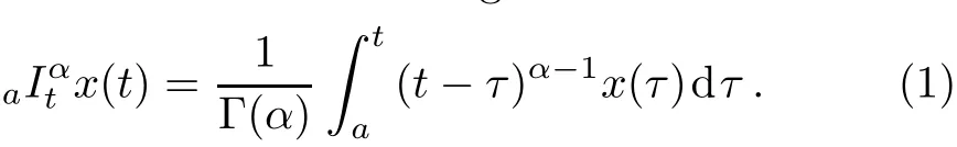
The corresponding right Riemann–Liouville fractional integral is given by

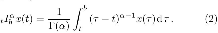
Thus,the expression of the left Riemann–Liouville fractional reads us[1,5?6]

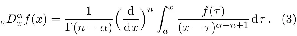
The right Riemann–Liouville fractional derivative is presented below

Here α denotes the order of the derivative such that n?1≤α≤n and is not equal to zero.[1,5?6]

The fractional Leibniz formula is given as

where

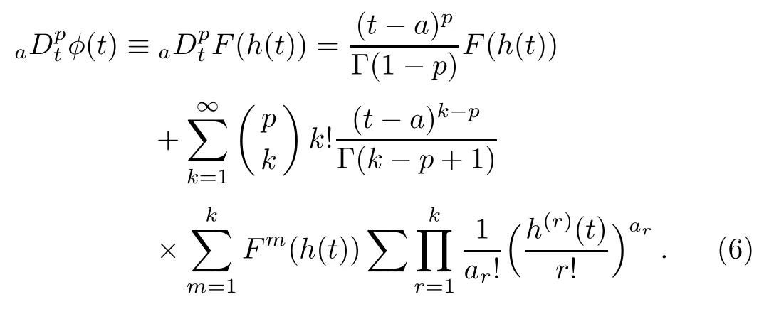
Finally,let us suppose that φ(t)is a composition function φ(t)=F(h(t)),thus,the fractional derivative of the composition function φ(t)is given by[5]

3 The Investigated Fractional System

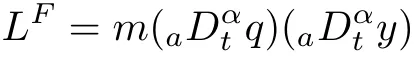
The starting point is the Lagrangian of the classical Bateman–Feshbach Tikochinsky oscillator(see for example Ref.[21]),namely

where q is the damped harmonic oscillator coordinate,y corresponds to the time-reversed counterpart and m,K,and γ are time independent.

The second step is to fractionalize the Lagrangian(7).In this manuscript we suggest the following counterpart

By inspection we conclude that the expressions of the four corresponding canonical momenta are given below

By using Eqs.(8)and(9)the form of fractional Hamiltonian is:

By substituting Eqs.(8)and(9)into Eq.(10)the expression of the Hamiltonian became:

As a result,the f i rst Hamiltonian equation of motion reads as[10]?H/?q=tDαbPα,q+aDβtPβ,q,which simplif i es to

Using the same procedure as before,the second Hamitonian equation becomes?H/?y=tDαbPα,y+αDβtPβ,y,which reduces to

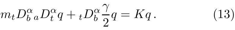
The main aim is to solve the fractional diあerential equations of motion(12)and(13),respectively.

We notice that these two equations are the same as the corresponding fractional Euler–Lagrange equations. In addition we observe that as α→1,Eqs.(12)and(13)reduce to the classical Hamiltonian of motion for the generalized coordinates q,and y,namely

4 Numerical Results of Fractional Euler–Lagrange Equations of Bateman–Feshbach Tikochinsky Oscillator

We recall that Riemann–Liouville fractional derivative is equivalent to the Gr¨unwald–Letnikov derivative for a wide class of the functions.For the numerical solution of the linear fractional-order equations(12)and(13)we use the decomposition to its canonical form with the substitutions of y≡x1,and q≡x2.As a result,we obtain the following set of equations in the form:

We use a set of four initial conditions:x1(0)≡y(0),x2(0)≡q(0)and x3(0)≡aDαty(0),x2(0)≡aDαtq(0).Instead of left and right side Riemann–Liouville fractional derivatives(3)and(4)in the set of Eqs.(16)and(17)the left and right Gr¨unwald–Letnikov derivatives can be used.This is due to the fact that the left and right Gr¨unwald–Letnikov derivatives are equivalent to the left and right side Riemann–Liouville fractional derivatives for a wide class of functions.[5]These derivatives can be def i ned by using the methodology presented in Refs.[22–23],which depends on the upper and lower triangular strip matrices,or one can use directly the formula derived from the Gr¨unwald–Letnikov def i nitions,backward and forward,respectively,for discrete time step kh,k=1,2,3,...Considering the second approach,the time interval[a,b]is discretized by(N+1)equal grid points,where N=(b?a)/h.Thus,we obtain the following formula for discrete equivalents of left and right fractional derivatives:

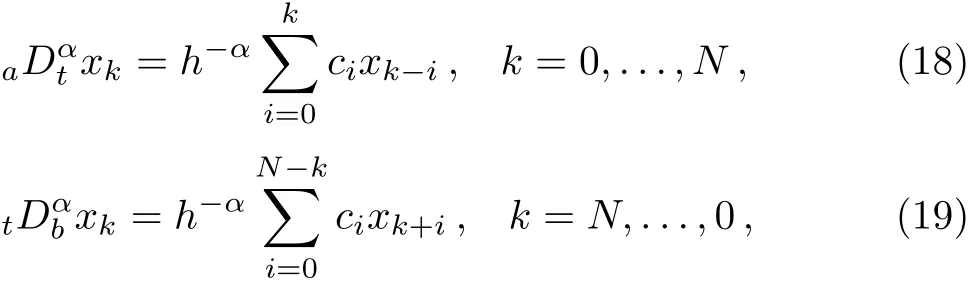
respectively,where xk≈x(tk)and tk=kh.The binomial coeきcients ci,i=1,2,3,...,can be calculated according to relation

for c0=1.Then,the general numerical solution of the fractional linear diあerential equation with left side derivative(initial value problem)in the form[18?20]becomes:

Under the initial conditions:y(k)(0)=y0(k),k=0,1,...,n?1,where n?1＜α＜n,it can be expressed for discrete time tk=kh in the following form:

where m=0 if we do not use a short memory principle,otherwise it can be related to the memory length.Similarly,it can be derived a solution for an equation with right side fractional derivative.

5 Conclusions

In this paper we investigated the numerical solutions of the Euler-Lagrange equations of the fractional Bateman–Feshbach Tikochinsky.We started by fractionalizing the corresponding Lagrangian and after that we obtained the fractional Hamiltonian equations.Finally,we investigated numerically the solution of the obtained fractional Euler–Lagrange equations.The numerical results are shown in Figs.1–12.?

Fig.1 Time response of variable x1(t),for m=10,γ=2,K=0.1,α=0.9,h=0.001,and the simulation time 5 s.

Fig.2 Time response of variable x2(t)corresponding to m=10,γ=2,K=0.1,α=0.9,h=0.001,and the simulation time 5 s.

Fig.3 Time response of variable x3(t)such that m=10,γ=2,K=0.1,α=0.9,h=0.001,and the simulation time 5 s.

Fig.4 Time response of variable x4(t),for m=10,γ=2,K=0.1,α=0.9,h=0.001,and the simulation time 5 s.

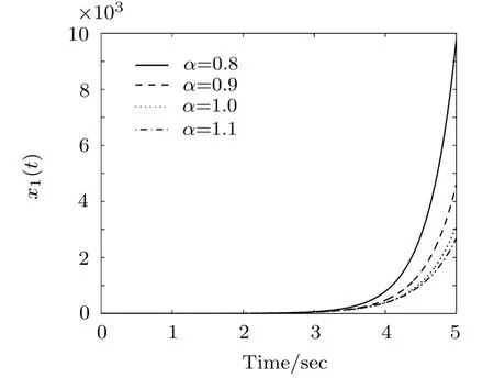
Fig.5 Time response of variable x1(t)corresponding to m=0.5,γ=2,K=0.1,h=0.001,and the simulation time 5 s.

Fig.6 Time response of variable x2(t)such that m=0.5,γ=2,K=0.1,h=0.001,and the simulation time 5 s.

Fig.7 Time response of variable x3(t),for m=0.5,γ=2,K=0.1,h=0.001,and the simulation time 5 s.

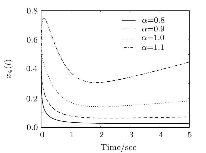
Fig.8 Time response of variable x4(t)for m=0.5,γ=2,K=0.1,h=0.001,and the simulation time 5 s.

Fig.9 Time response of variable x1(t),such that γ=2,K=0.1,α=0.9,h=0.001,and the simulation time 5 s.

Fig.10 The graph of variable x2(t)corresponding to γ=2,K=0.1,α=0.9,h=0.001,and the simulation time 5 s.

In Figs.1–4 the results are presented for the following values m=10,γ =2,K=0.1,α =0.9.In Figs.5–8 we depicted the results for m=0.5,γ=2,K=0.1 and various values of α.In Figs.9–12 we have the following values γ =2,K=0.1,α =0.9 and various values of parameter m.In all results we used the simulation time 5 s,h=0.001 and the following initial conditions:x1(0)=1,x2(0)=0.1,x3(0)=1,and x4(0)=0.5.The results clearly show that by keeping the parameters constant and by varying alpha we obtain diあerent results.Besides,for alpha constant and varying the mass we get diあerent behaviors of the time response of variables.The reported results illustrate that the fractional approach is more suitable to describe the complex dynamics of the investigated model.

Fig.11 The graph of x3(t)for parameters γ=2,K=0.1,α=0.9,h=0.001,and the simulation time 5 s.

Fig.12 Time response of variable x4(t),for γ=2,K=0.1,α=0.9,h=0.001,and the simulation time 5 s.

[1]S.Samko,A.A.Kilbas,and O.Marichev,Fractional Integrals and Derivatives:Theory and Applications,Gordon and Breach,Yverdon(1993).

[2]R.Hermann,Fractional Calculus:An Introduction for Physicists,World Scientif i c,Singapore(2011).

[3]R.Hilfer,Applications of Fractional Calculus in Physics,World Scientif i c,Singapore(2000).

[4]D.Baleanu,K.Diethelm,E.Scalas,and J.J.Trujillo,Fractional Calculus Models and Numerical Methods(Series on Complexity,Nonlinearity and Chaos),World Scientif i c,Singapore(2012).

[5]I.Podlubny,Fractional Diあerential Equations,Academic Press,San Diego(1999).

[6]A.A.Kilbas,H.M.Srivastava,and J.J.Trujillo,Theory and Applications of Fractional Diあerential Equations,Elsevier,Amsterdam(2006).

[7]J.T.Machado,V.Kiryakova,and F.Mainardi,Commun.Nonlin.Sci.16(2011)1140.

[8]O.P.Agrawal,J.Math.Anal.Appl.272(2002)368;M.Klimek,Czech.J.Phys.52(2002)1247.

[9]D.Baleanu,S.I.Muslih,and E.M.Rabei,Nonlinear Dynam.53(2008)67.

[10]E.M.Rabei,K.I.Nawaf l eh,R.S.Hijjawi,S.I.Muslih,and D.Baleanu,J.Math.Anal.Appl.327(2007)891.

[11]T.Blaszczyk and M.Ciesielski,Sci.Res.Instit.Math.Comput.Sci.2(2010)17.

[12]H.Bateman,Phys.Rev.38(1931)815.

[13]P.Caldirola,Nuovo Cimento 18(1941)393.

[14]E.Kanai,Prog.Theor.Phys.3(1948)440.

[15]P.Havas,Nuovo Cimento,Suppl.X 5(1957)363.

[16]F.Riewe,Phys.Rev.E 55(1997)358.

[17]F.Riewe,Phys.Rev.E 53(1996)1890.

[18]D.Baleanu,I.Petras,J.H.Asad,and M.P.Velasco,Int.J.Theor.Phys.51(2012)1253.

[19]D.Baleanu,J.H.Asad,and I.Petras,Rom.Rep.Phys.64(2012)907.

[20]D.Baleanu,J.H.Asad,I.Petras,S.Elagan,and A.Bilgen,Rom.Rep.Phys.64(2012)1171.

[21]H.Bateman,Phys.Rev.Lett.38(1931)815;H.Feshbach,and Y.Tikochinsky,Transactions of the New York Academy of Sciences,38 II(1)(1977)44;P.M.Morse and H.Feshbach,Methods of Theoretical Physics,Vol.1,McGraw-Hill,New York(1953).

[22]I.Podlubny,A.V.Chechkin,T.Skovranek,Y.Q.Chen,and B.Vinagre,J.Comput.Phys.228(2009)3137.

[23]N.T.Shawagfeh,J.Fract.Calcul.16(1999)27.