
NONLINEAR STABILITY OF RAREFACTION WAVES FOR A COMPRESSIBLE MICROPOLAR FLUID MODEL WITH ZERO HEAT CONDUCTIVITY?
2020-11-14 09:41:12JingJIN金晶NoorREHMAN2QinJIANG江芹
Jing JIN (金晶)1? Noor REHMAN2 Qin JIANG (江芹)1
1. School of Mathematics and Statistics, Huanggang Normal University, Huanggang 438000, China
2. School of Mathematics and Statistics, Central China Normal University, Wuhan 430079, China
E-mail : jinjing@hgnu.edu.cn; noorwzr786@gmail.com; 113572710@qq.com
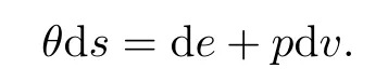
We assume, as is usual in thermodynamics, that by using any given two of the five thermodynamical variables – v,p,e,θ, and s – the remaining three variables are their functions.Furthermore, their relation is implied by the second law of thermodynamics:
According to this, if we choose (v,θ) as independent variables and write (p,e,s) = (p(v,θ),e(v,θ),s(v,θ)), then we can deduce that
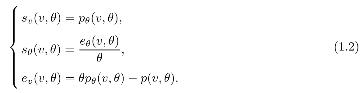
Therefore, the energy equation (1.1)3can be converted into the equations for the entropy s or the absolute temperature θ by the second law of thermodynamics as follows:

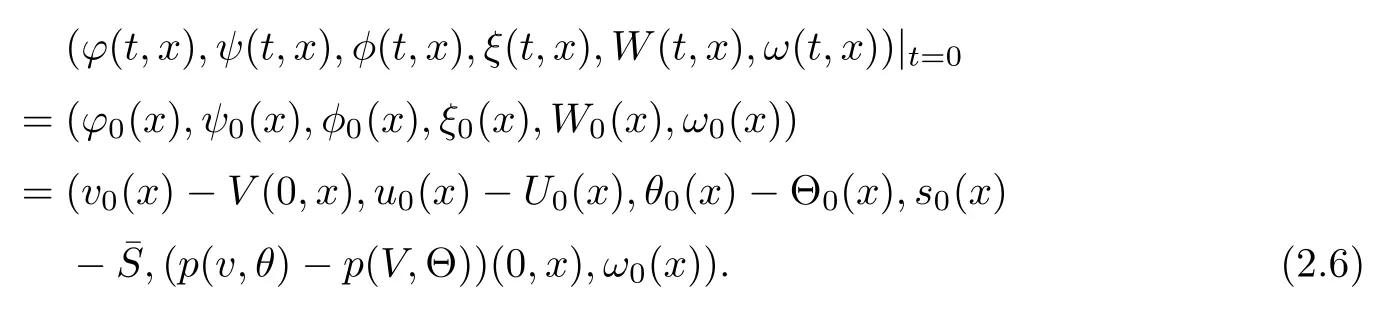
We supplement this system with the initial condition

The corresponding initial data at far field x=±∞are given by

where we assume that ω?= ω+=0.
Large time behavior was considered in[8–10],which studied the local stability of rarefaction waves, contact waves and viscous shocks wave when heat conductivity is a positive constant.
We note that all of the above analyses take advantage of the fact that the entropy is dissipative,because of the non-zero heat conductivity. However,in this article,we are concerned with the time-asymptotic stability of rarefaction waves to the Cauchy problems(1.1),(1.5)and(1.6), with zero heat conductivity (κ = 0). On account of the lack of heat conductivity,the estimates of the termwhich plays an essential role in closing the energy estimates,could hardly be obtained by applying the usual L2-energy estimates. Hence we could not apply the method of [9]here. However, in [1], inspired by [11], the author successfully closed the energy estimates by considering the equations as a system of unknowns relating to pressure, velocity and entropy, instead of system relating to unknowns of density, velocity and temperature.
In this article, we consider the polytropic gas that admits

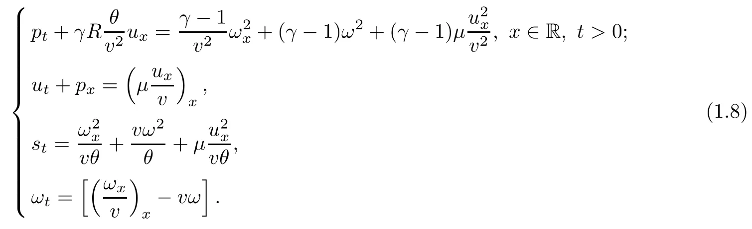
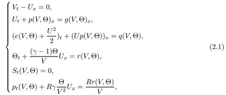
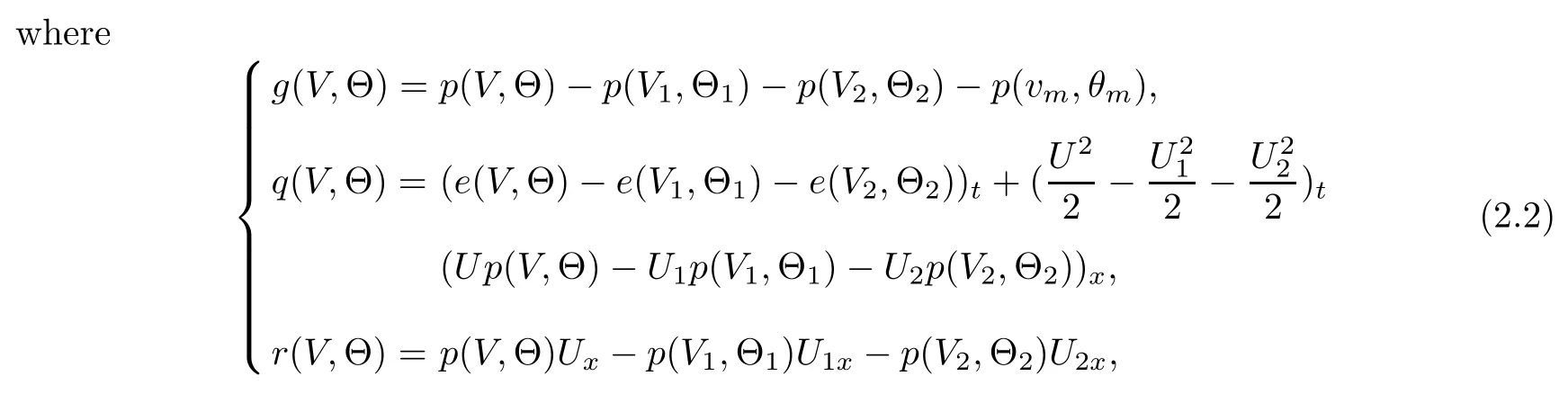
Here the specific gas constants A, R and the specific heat at constant volume Cvare positive constants, and γ > 1 is the adiabatic constant. Inspired by [1], we first convert (1.1) into the system of pressure, velocity and entropy as follows:
As we will focus on the expansion waves, we assume in the rest of this article that s+=s?=. According to Darcy’s law, we see from (1.11)4that ω → 0 as t → ∞. Therefore the system should tend time-asymptotically to
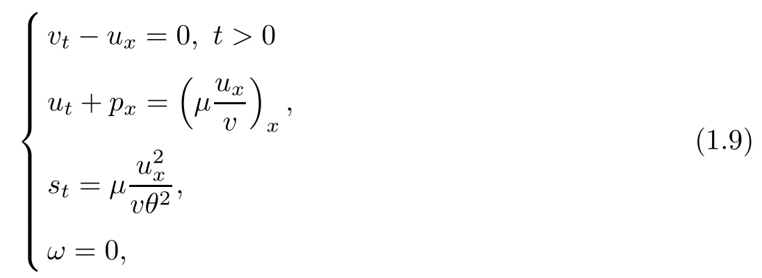
where we see that the first three equations in (1.9) happen to be non-isentropic Navier-Stokes equations, and combined with the initial data (1.6), they should tend time-asymptotically to the Riemann problem on a Euler system in the setting
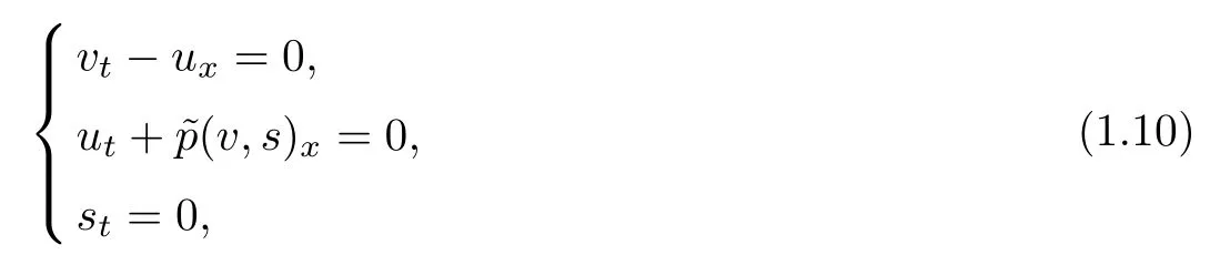
with Riemann data
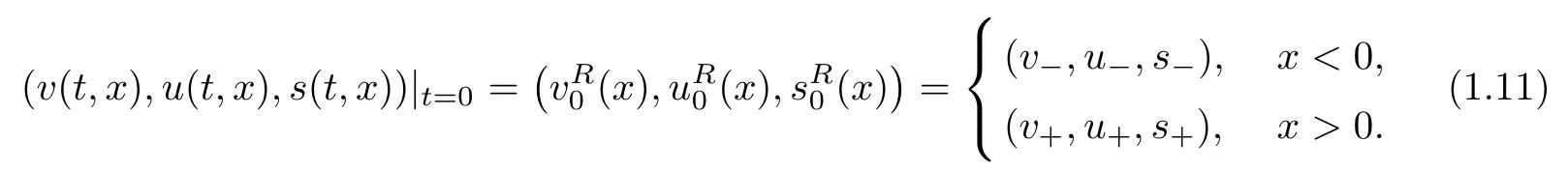
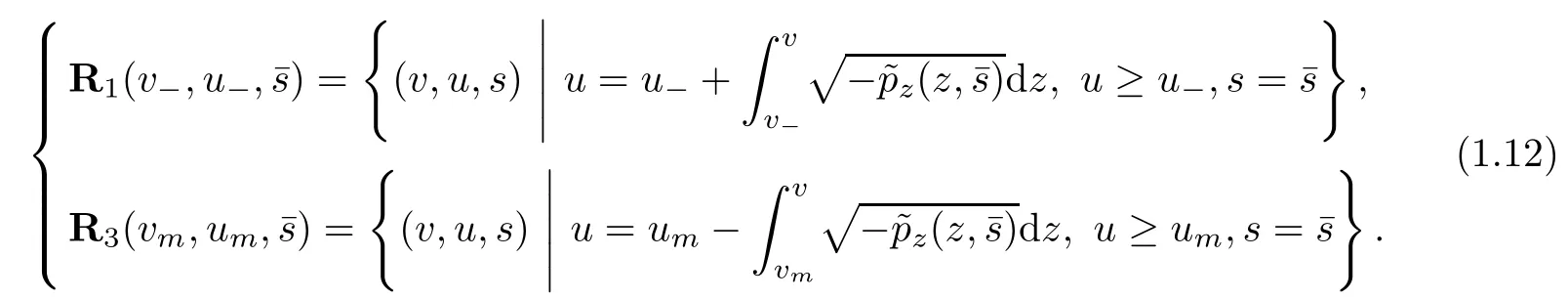
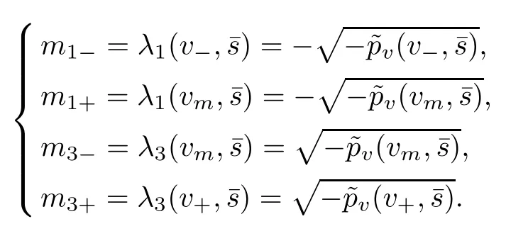
We consider the case when the Riemann problem(1.10),(1.11)admits a unique global weak(rarefaction wave)solutionwhich consists of a rarefaction wave of the first family, denoted byand another of the third family, denoted byThat is, there exists a unique constant state (vm,um) ∈R2(vm> 0)such that (vm,um)∈ R1(v?,u?) and (v+,u+)∈ R3(vm,um). Here,
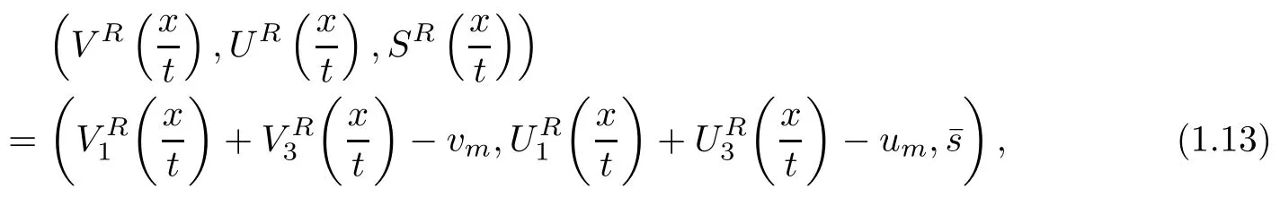
In other words, the unique weak solutionto the Riemann problem(1.10) and (1.11) is given by

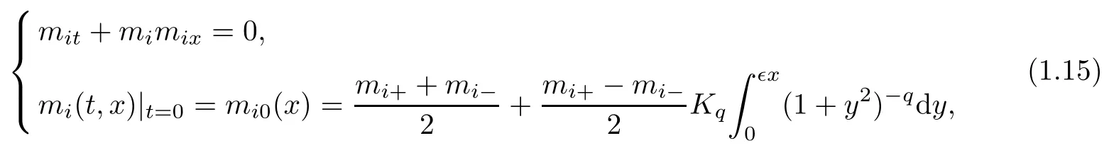
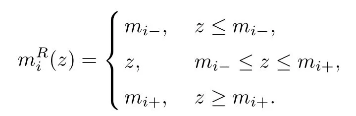
To study the above problem,as in [12]and[13],we first construct a smooth approximation to the above Riemann solution (1.13). Let mi(t,x) (i = 1,3) be the unique global smooth solution to the Cauchy problem
Then, by setting ? = δ = |v?? v+|+|u?? u+|, the smooth approximation of the rarefaction wave profile (V(t,x),U(t,x),S(t,x)) is constructed as follows:

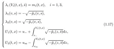
Here, (Vi(t,x),Ui(t,x)) (i=1,3) are given by the equations
and Θ is defined by

Under the above preparation, for the ideal polytropic gas, our nonlinear stability result on the rarefaction wave VR(t,x),UR(t,x),SR(t,x),0 can be stated as follows:
Theorem 1.1(Nonlinear Stability) Assume that VR(t,x),UR(t,x),SR(t,x),0 is the solution to the Riemann problem of the compressible Euler equations (1.10),(1.9)4and (1.11),given by(1.13),and that the initial data(v0(x),u0(x),s0(x),ω0(x))of the compressible micropolar equations (1.8) satisfies (1.6), and that
for all (t,x)∈ R+×R and some positive constantsLet

denote the H2(R)-norm of the initial perturbation and let δ = |u?? u+|+|v?? v+| denote the strength of rarefaction wave. If E(0) and δ are suitably small such that
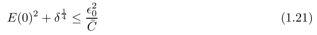
for a positive constant ?0>0, whereis a constant depending only onwhich will be defined at the end of this article,then the Cauchy problem(1.1)1,(1.8)2,(1.8)3,(1.8)4,(1.5)and (1.6) admits a unique global solution (v(t,x),u(t,x),θ(t,x),ω(t,x)) satisfying

Remark 1.2Due to the assumption that the initial perturbation E(0) and the strength of the rarefaction wave δ are suitably small, the result obtained in Theorem 1.1 is essentially the local stability of weak rarefaction waves.
Now we would like to make two comparisons in order to point out the main novelties of this article. First, compared with [1], where the initial data (v0(x),u0(x),s0(x),ω0(x)) is a perturbation of a non-vacuum constant state, the main difficulty confronted in this article is determining how to control the possible growth of the solution of Cauchy problem (1.8), (1.5)and (1.6) induced by the interactions between the solution itself and the underlying expansive waves from different families. Such a difficulty is overcame by the expansive property and the temporal decay estimates of the smooth approximation of the rarefaction waves. Secondly,compared with [9](where μ > 0, κ > 0), which studied the nonlinear stability of rarefaction waves to the Cauchy problem of(1.1),(1.6), in our paper,even the basic energy type estimates cannot be closed, and we introduce another functional E(t) defined by (3.3) to deduce the desired estimate; see the proof of Lemma 4.1.
Before concluding this section, we first recall that the study on compressible Micropolar fluid has become an important area of interest for theoretical mathematicians. For the one dimensional case on the existence, uniqueness and regularity of either the Cauchy problem or the initial-boundary problems, we refer to [4, 5, 14–25]and the references therein. In addition,just as the dissipation effect of heat conductivity is neglected in this article, there is another work that considers the large time behavior without the dissipation effect of viscosity [26].For the three dimensional case on the existence, uniqueness, large time behavior and decay rate, blow up criterion and low mach number limit for either the Cauchy or initial-boundary problems,we refer to[27–41]and the references therein. Here,we also recall the classical works on the stability and vanishing viscosity limit on the rarefaction waves [42–56], which give us a deeper understanding of these elementary waves.
This article is arranged as follows: in Section 2, we give some properties of the smooth approximation of the rarefaction wave solutions and reformulate the problem. In Section 3, we state the main result for the reformulated problem and prove the main theorem by combining the local existence and the a priori estimates. Finally, the a priori estimates are established in Section 4.
NotationsThroughout the rest of this article,C or O(1)will be used to denote a generic positive constant independent of t and x,and Ci(·,·)(i ∈ Z+)stands for some generic constants depending only on the quantities listed in parenthesis. Note that all these constants may vary from line to line. Hl(R)(l ≥ 0) denotes the usual Sobolev space with normandwill be used to denote the usual L2-norm. For 1 ≤ p ≤ +∞, f(x) ∈ Lp(R,Rn),It is easy to see thatFinally,are used to denoterespectively.
2 Preliminaries
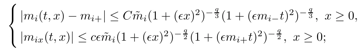
Lemma 2.1For each i ∈{1,3}, the Cauchy problem (1.15) admits a unique global smooth solution mi(t,x) which satisfies the following properties:
(i) m?
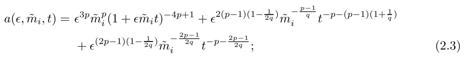
(ii) For any p with 1 ≤ p ≤ ∞, there exists a constant Cp,q, depending only on p,q, such that
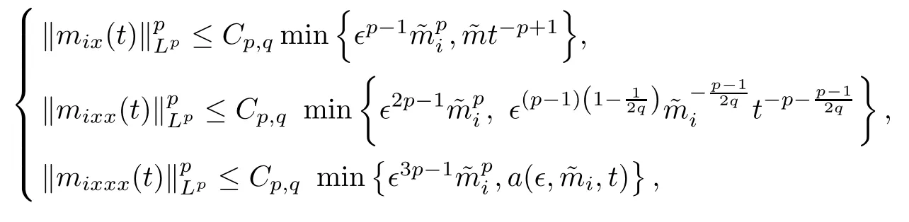
where
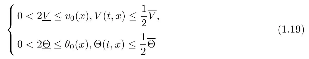
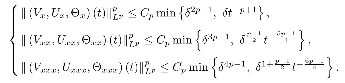
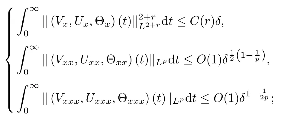
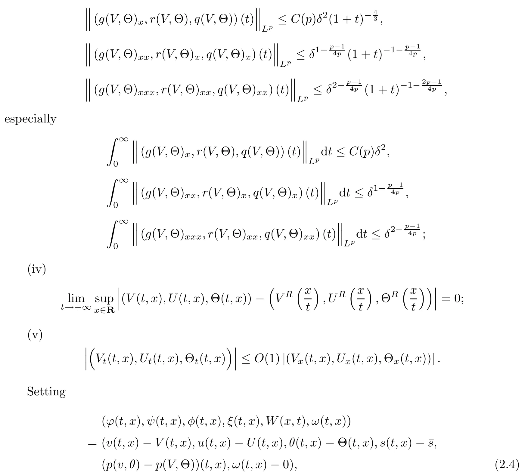
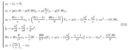
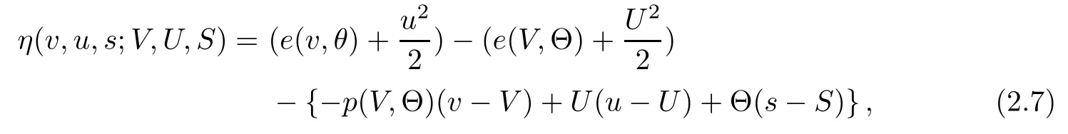
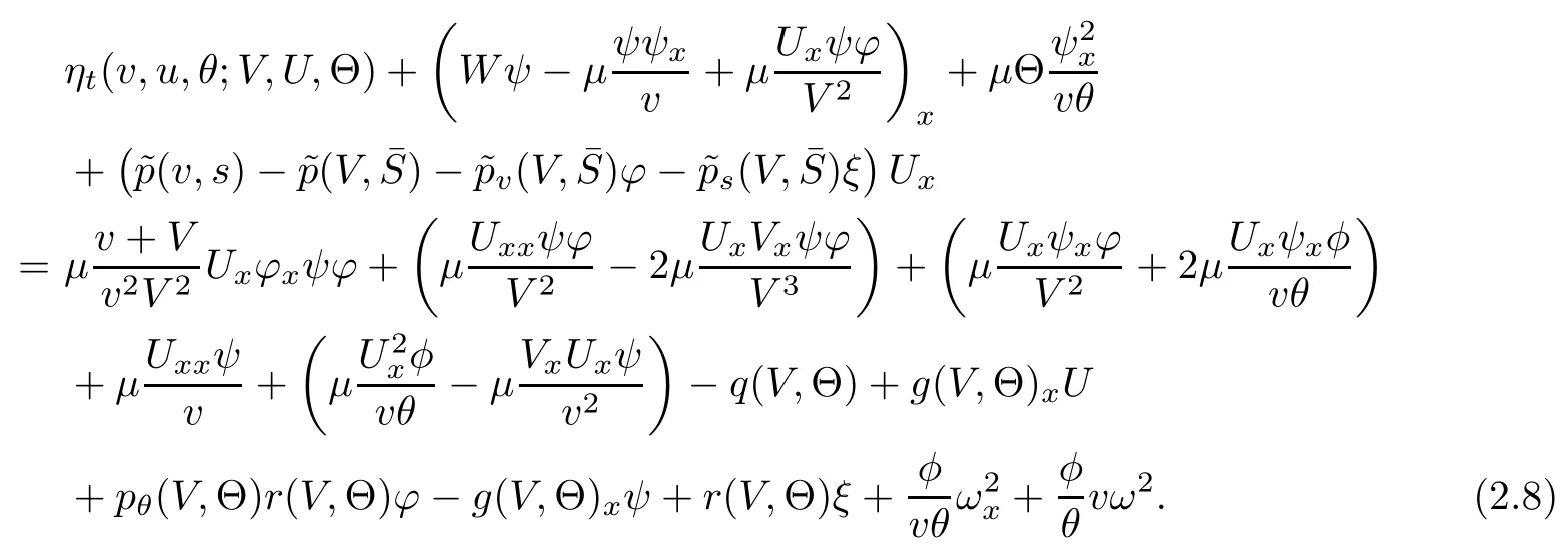
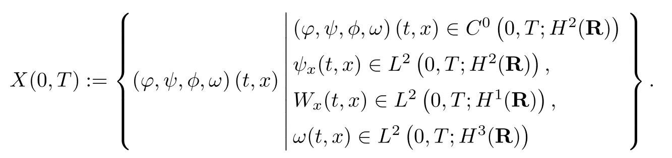
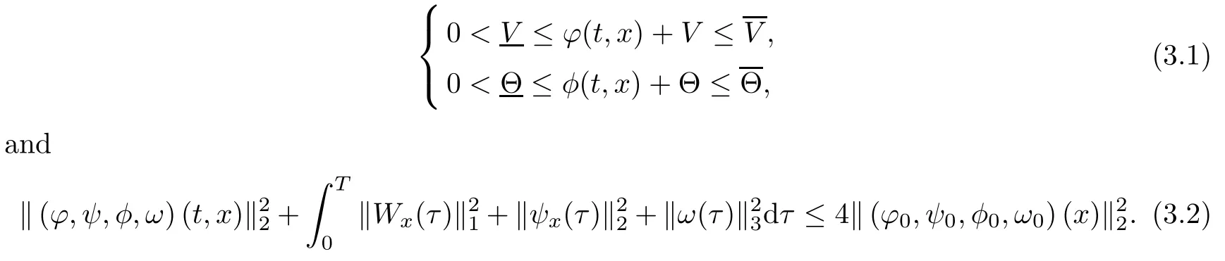
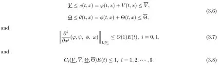
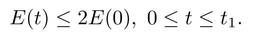
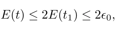
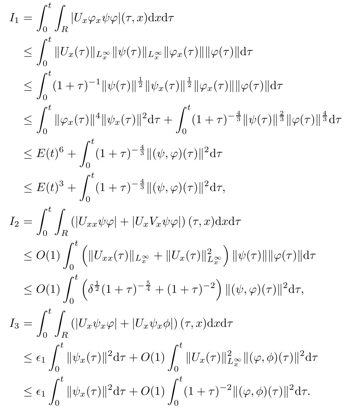
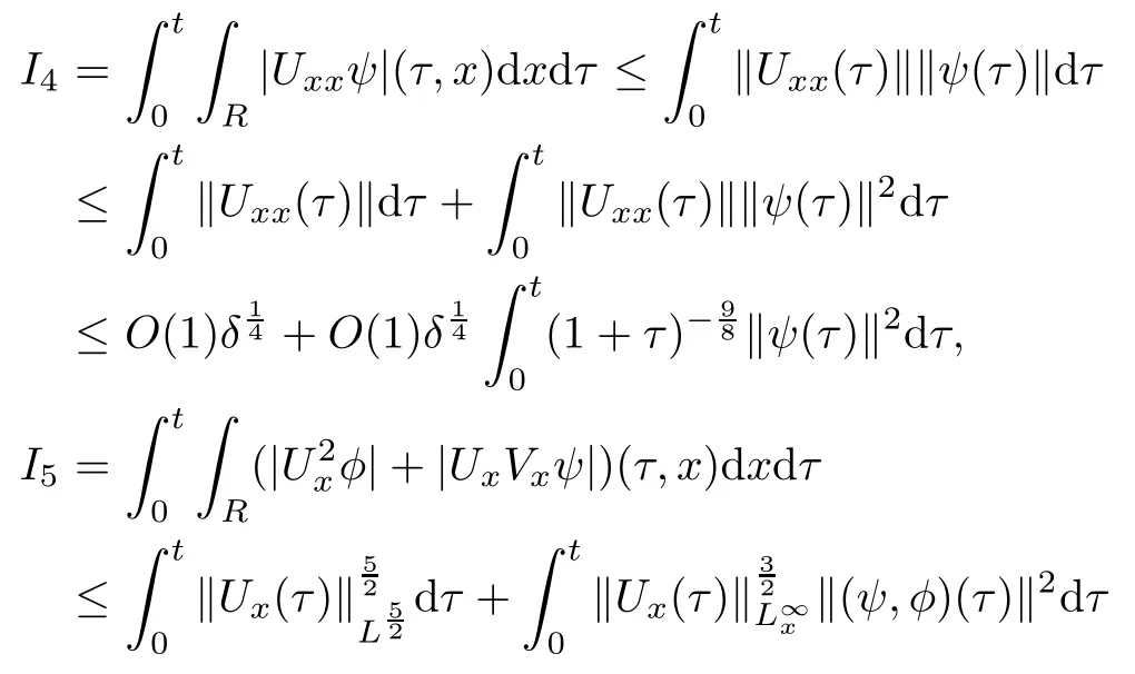
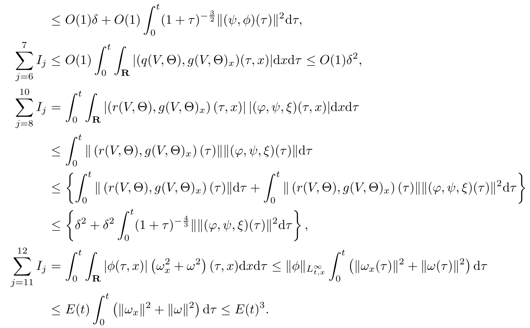
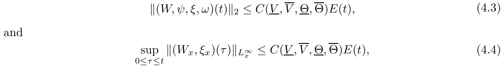
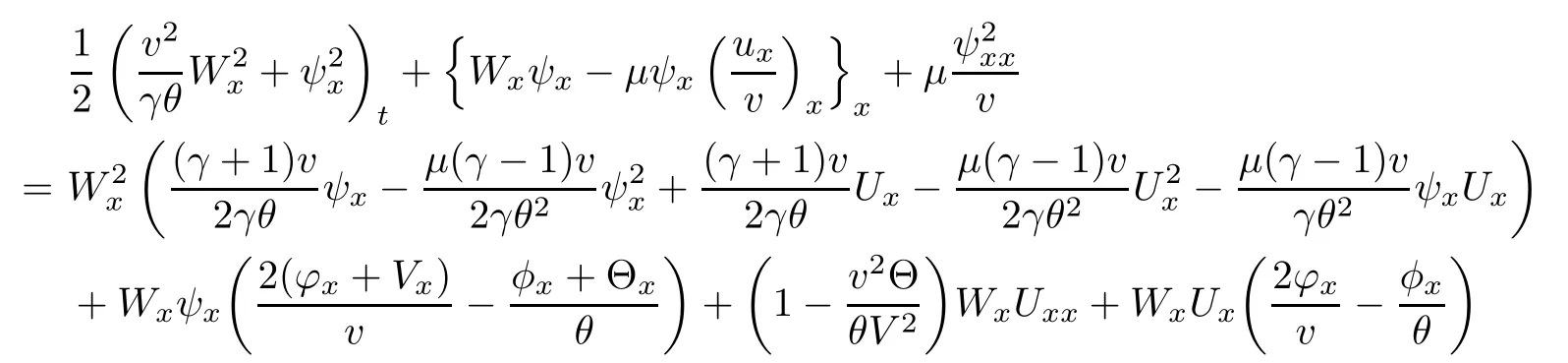
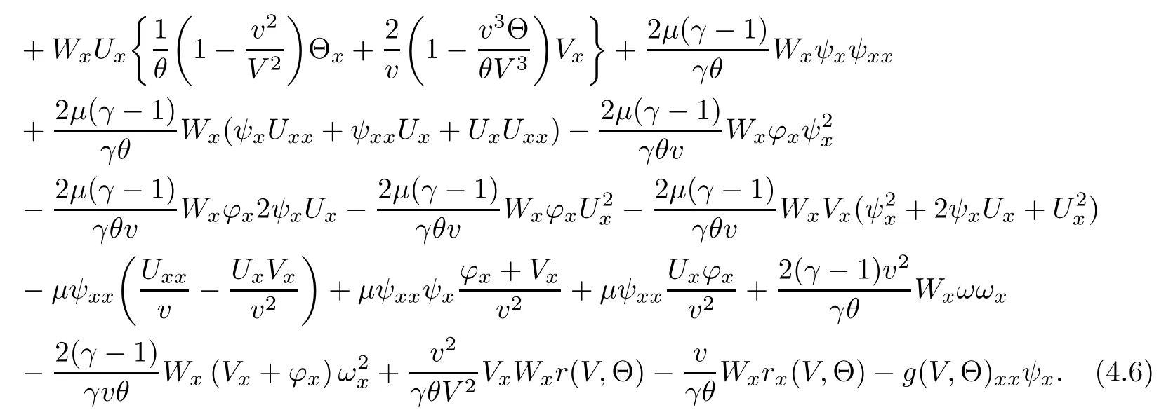
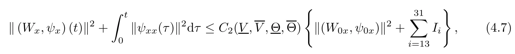
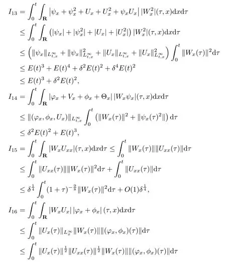
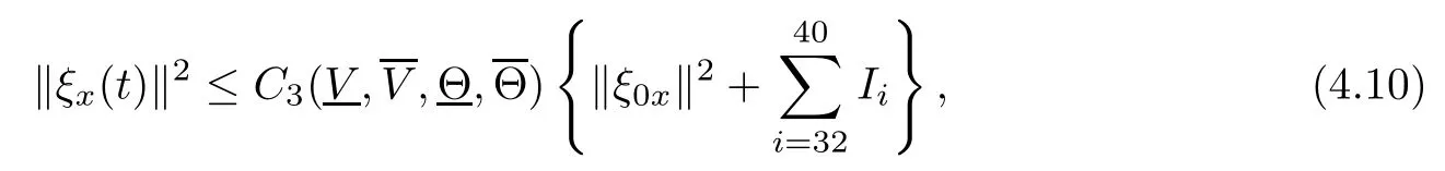
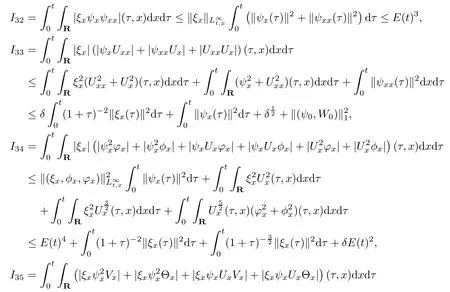
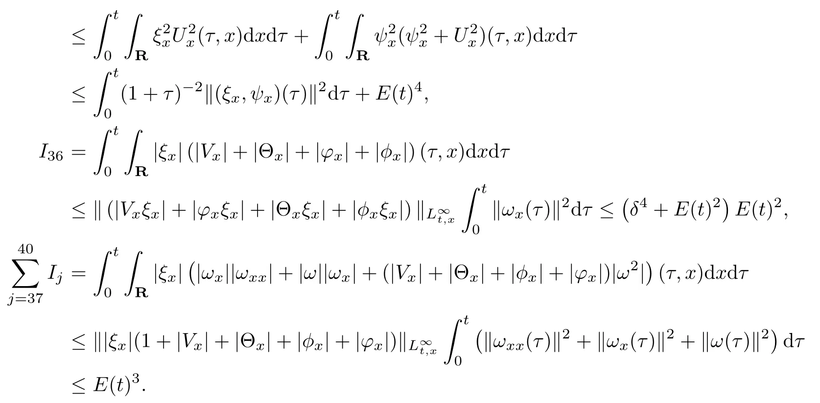
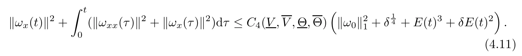
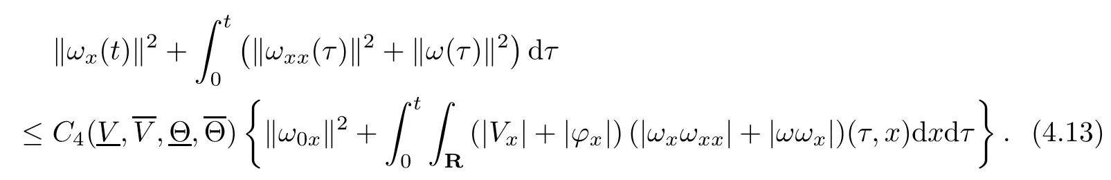
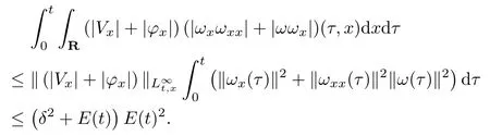
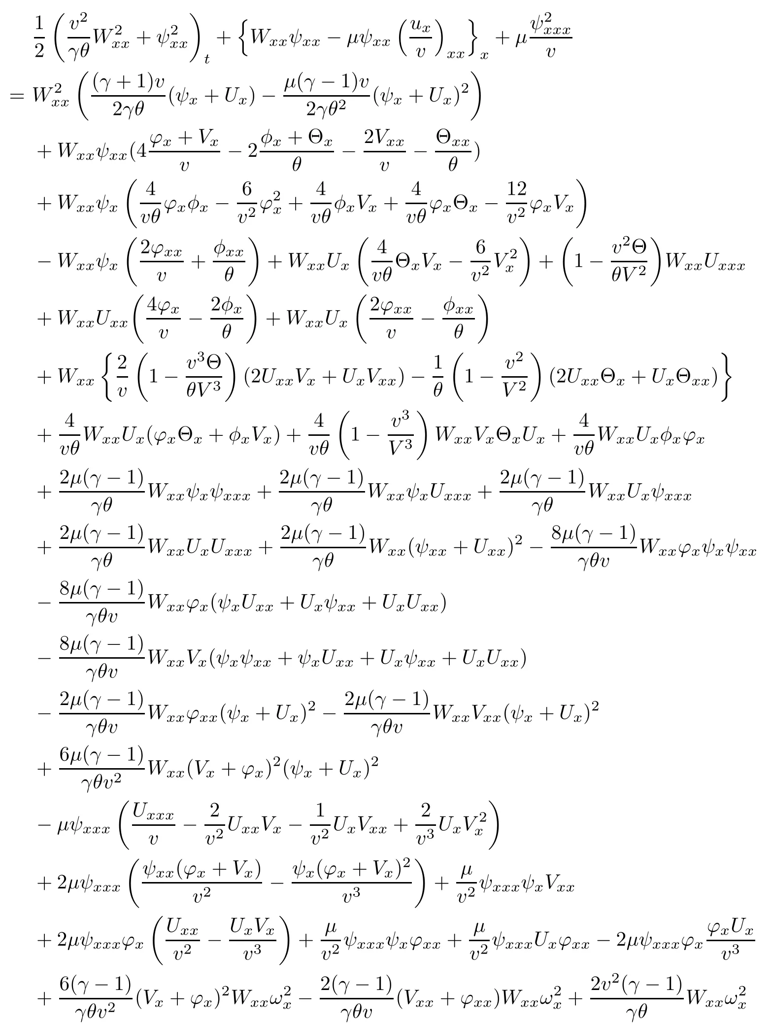
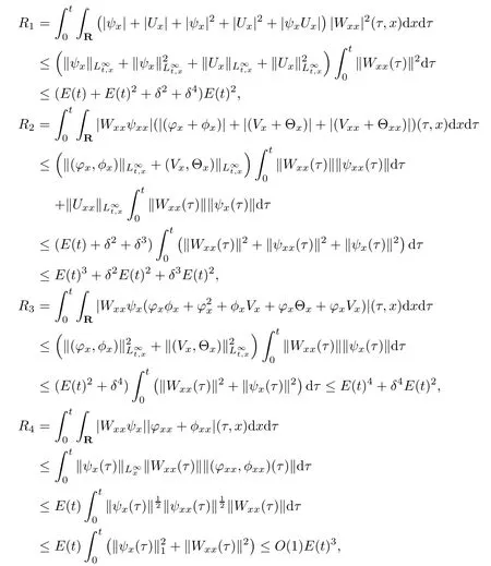
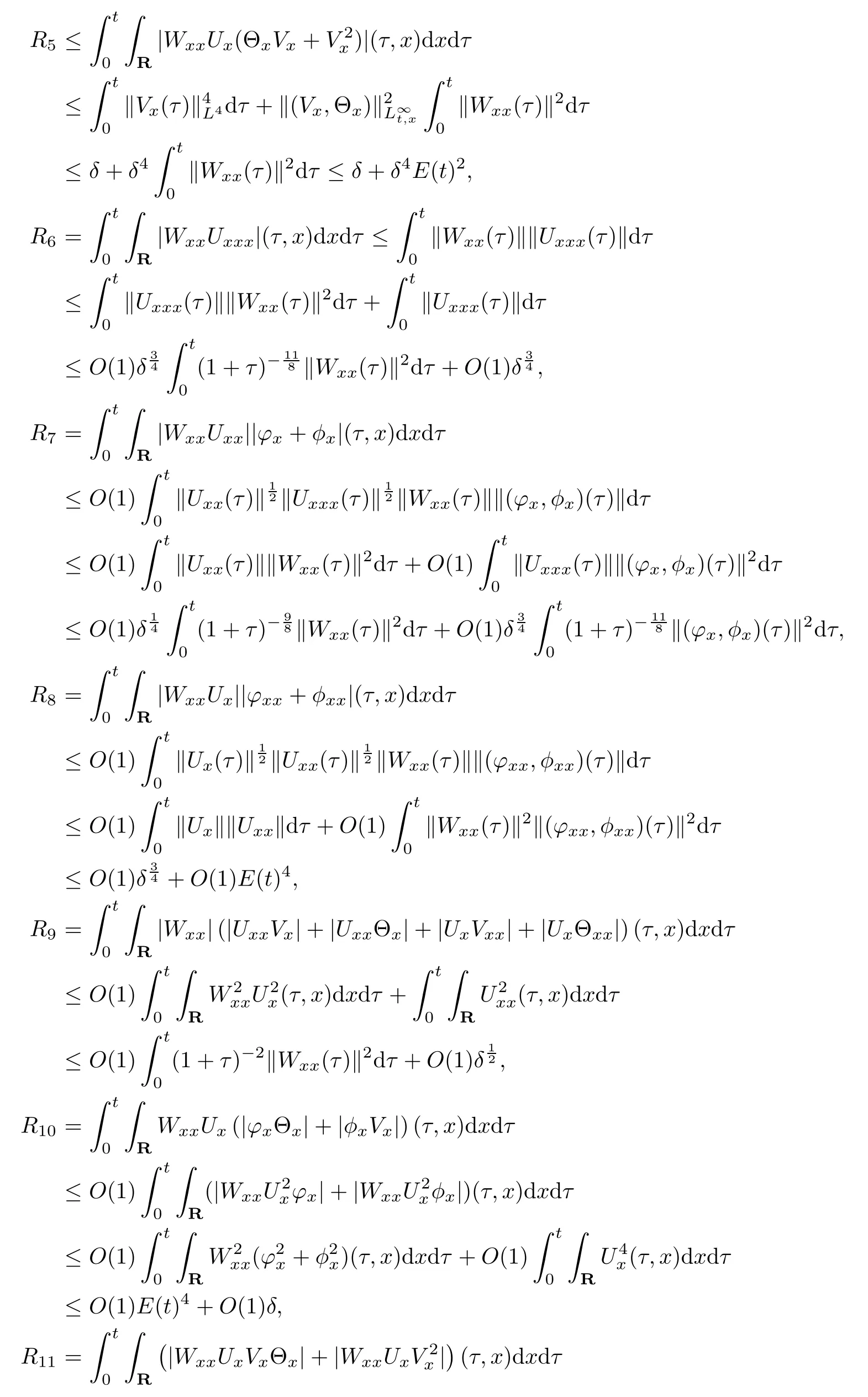
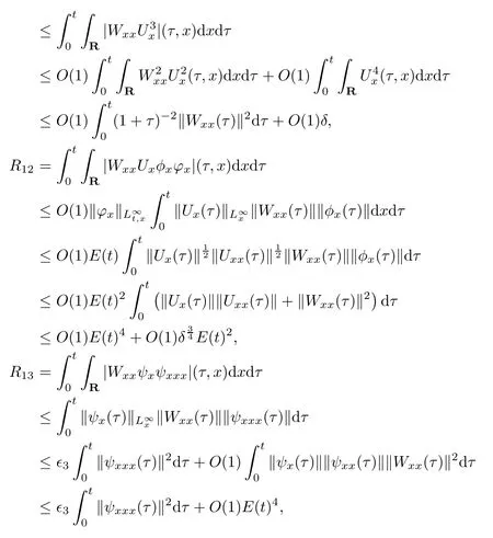
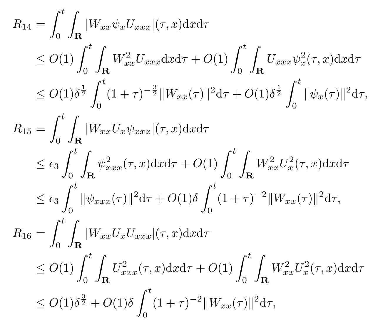
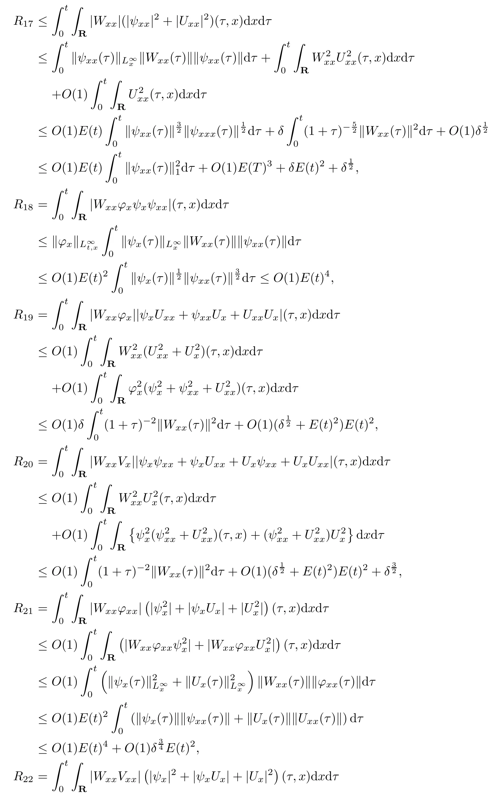
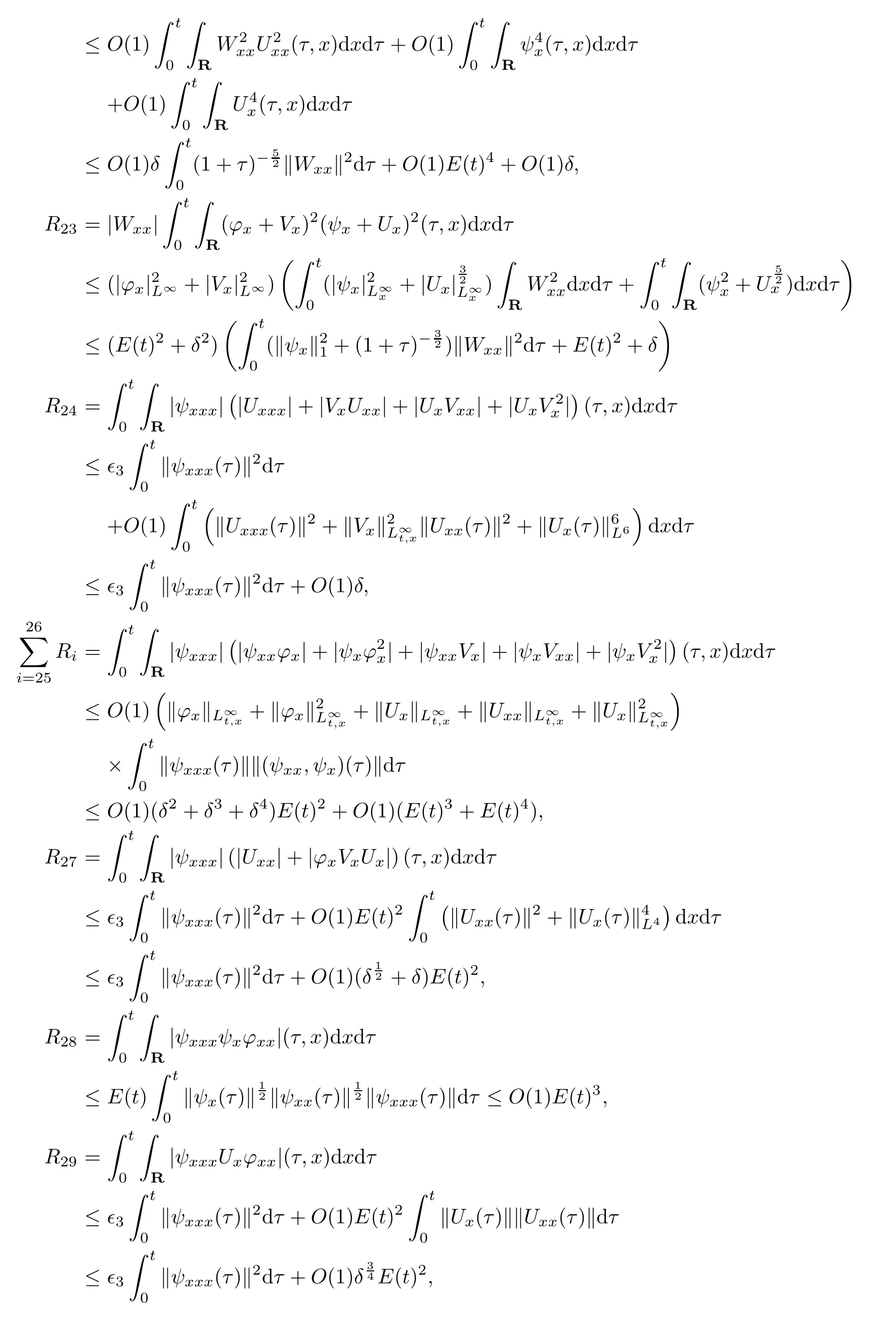
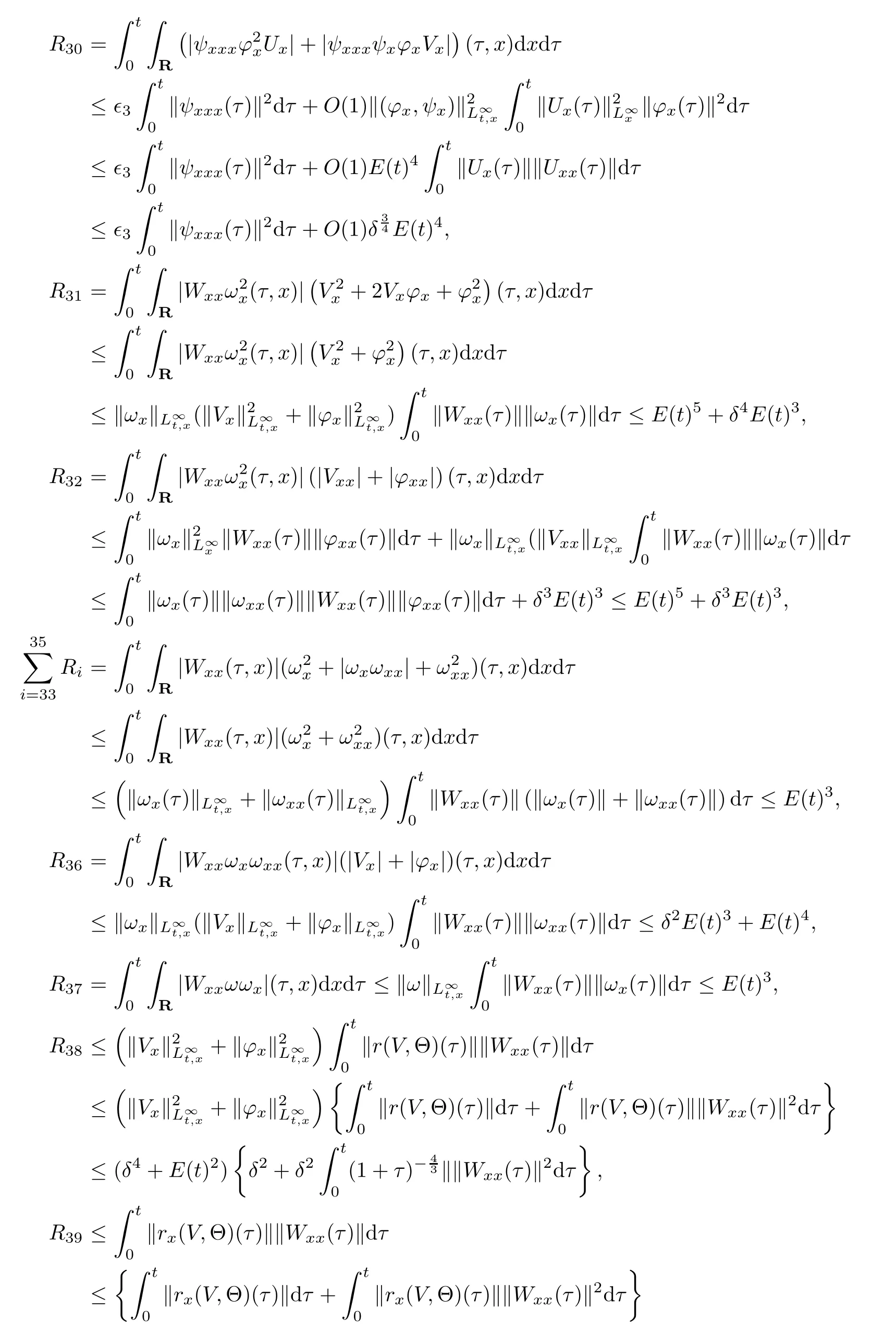
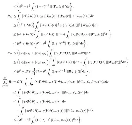
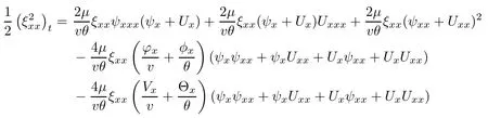
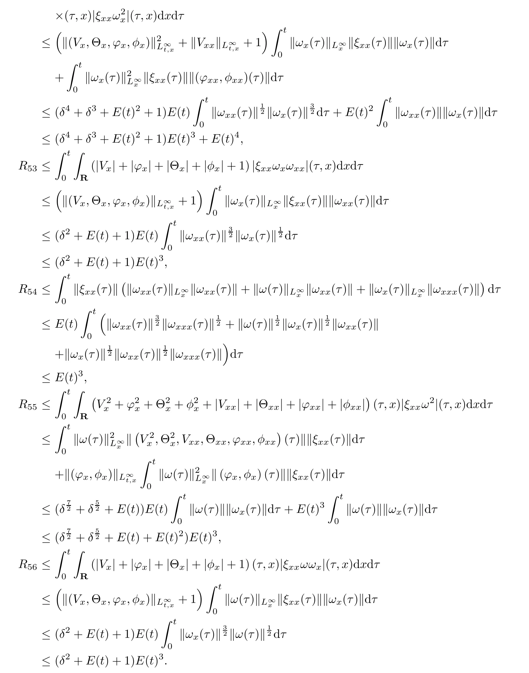
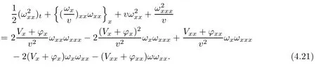
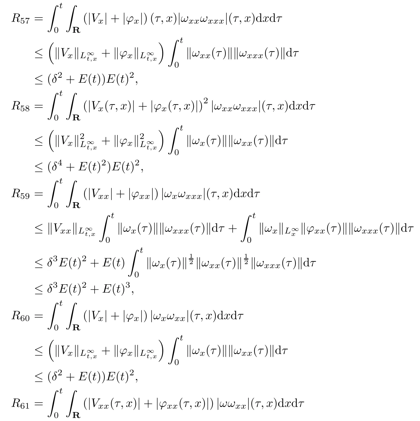
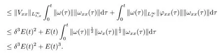
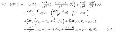
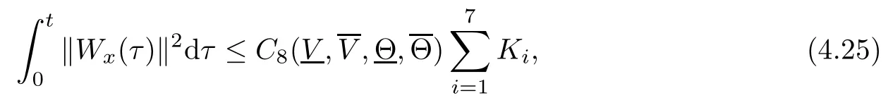
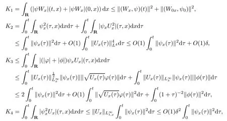
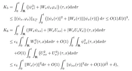
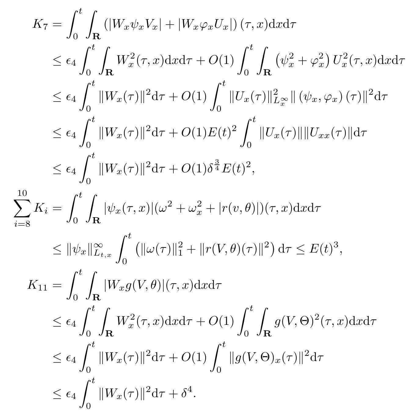
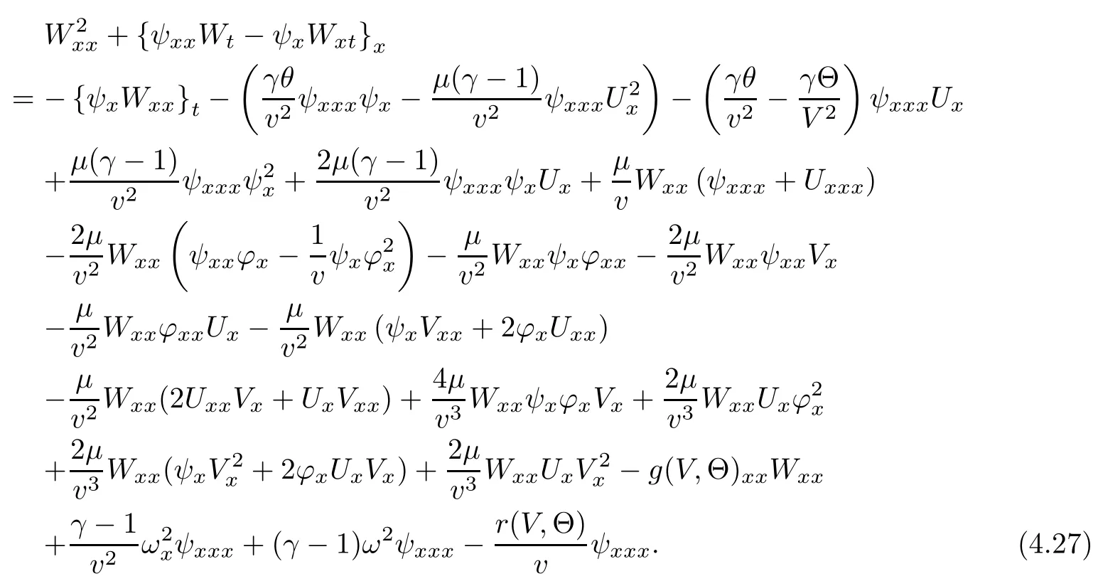
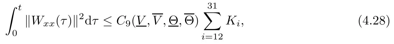
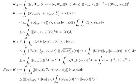
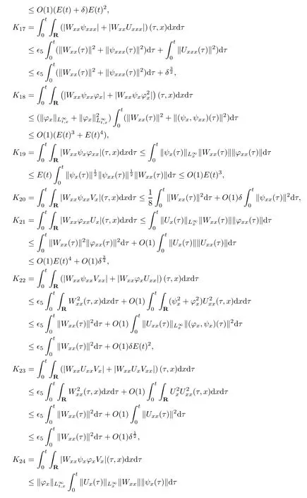
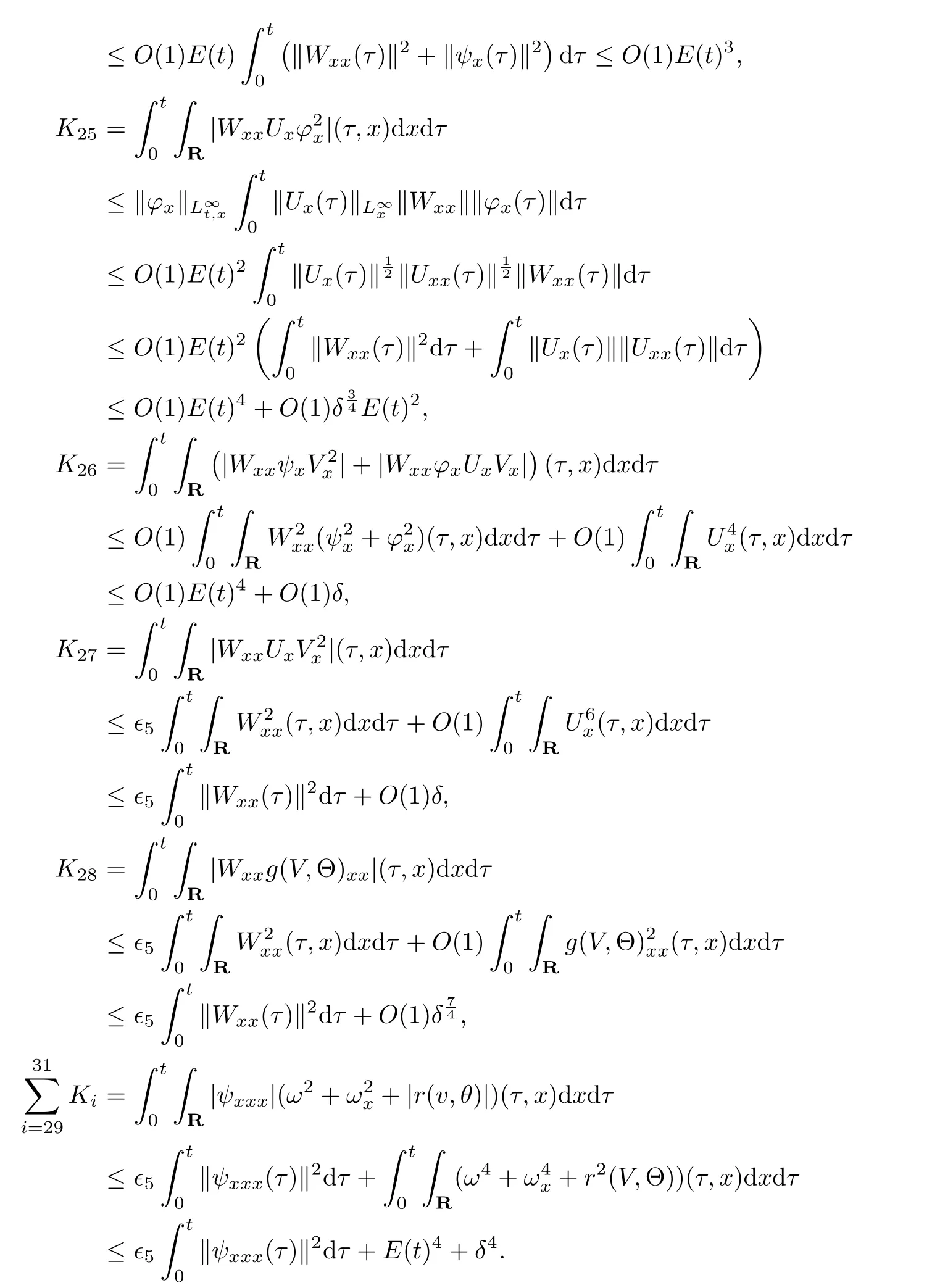
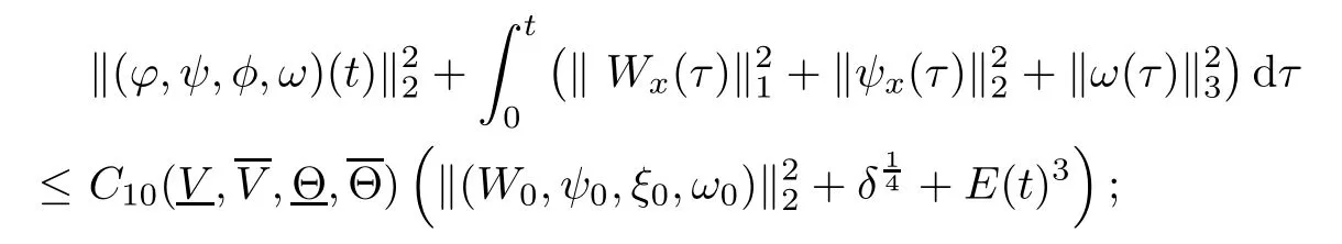
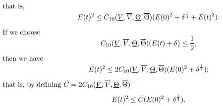
(iii) If 0 (iv) If (mi?) Based on the results obtained in Lemma 2.1, and from (1.16) and (1.17), we can deduce Lemma 2.2Letting ? = δ, q = 2, the smooth approximation (V(t,x),U(t,x),Θ(t,x))constructed in (1.16) and (1.17) has the following properties: (i) Vt(t,x)=Ux(t,x)>0 for each (t,x)∈R+×R; (ii) For any p with 1 ≤ p ≤ ∞ there exists a constant Cp, depending only on p, such that (iii) For each p ≥1, we deduce that (?(t,x),ψ(t,x),φ(t,x),ξ(t,x),W(t,x), ω(t,x)) yield with initial data Here we note that(2.5)i(i=1,2,3,6)and the corresponding initial data in(2.6)have formed a closed system, and that this is equivalent to (2.5)i(i=2,4,5,6)with the corresponding initial data. We write these together in order to facilitate future use. Define the following normalized entropy η(v,u,s;V,U,S) around (V(t,x),U(t,x),S(t,x)): which yields the entropy identity This section is devoted to proving Theorem 1.1. For convenience of presentation, in what follows we will choose(?,ψ,φ,ω) as independent variables,and for some fixed T >0,we define the solution space of (2.5)i(i=1,2,3,6) and the corresponding data in (2.6) by Then, a standard contracting-mapping argument (cf. [5]) yields the following local existence result: Proposition 3.1(Local existence result) Under the assumptions stated in Theorem 1.1, the Cauchy problem (2.5)i(i = 1,2,3,6), (2.6) admits a unique solution ?(t,x),ψ(t,x),φ(t,x),ω(t,x) ∈ X(0,t1)for some sufficiently small t1>0,and ?(t,x),ψ(t,x),φ(t,x),ω(t,x) satisfies Here t1depends only on To extend the local solution obtained in Proposition 3.1 globally, we need only to get the H2-norm a priori estimates on the solution that can be stated in the following: Proposition 3.2Under the assumptions stated in Theorem 1.1, suppose that (?(t,x),ψ(t,x),φ(t,x),ω(t,x)) obtained in Proposition 3.1 has been extended to the time t=T ≥ t1–that is, (?(t,x),ψ(t,x),ξ(t,x),ω(t,x)) ∈ X(0,T) – and satisfies the a priori assumption for some positive constant ?0>0. Then we can obtain the energy estimate in the form Remark 3.3If we have obtained (3.4), then by choosing the initial perturbation E(0)=and δ = |v?? v+|+|u?? u+| sufficiently small such that (1.21) holds, we can deduce that E(t) ≤ 2?0for 0 < t ≤ T. This implies that the a priori assumption (3.3)makes sense. Remark 3.4In fact, from (3.3) and (1.19), we have, from Sobolev’s inequality and by choosing ?0>0 suitably small, (3.6), (3.7) and (3.8) will be used in the proof of Proposition 3.2. The proof is a combination of a sequence of energy estimates that will be given at the end of Section 4. Now we are ready to extend the local solutions to global ones,that is the proof of Theorem 1.1 by a continuity argument. Proof of Theorem 1.1First,we take the time t=0 as initial data. Employing the local existence result Proposition 3.1, there exists a positive constant=t1(E(0)) > 0 , which depends only on E(0), such that there exists a unique solution ?(t,x),ψ(t,x), φ(t,x),ω(t,x)∈ X(0,t1) to (2.5)i(i=1,2,3,6) and (2.6) satisfying By the assumption on E(0) stated in Theorem 1.1, we have and then we have from Proposition 3.2 that for 0 ≤ t ≤ t1, By (3.10) and the assumptions (1.21), we observe that for 0 ≤ t ≤ t1, that is, for 0 ≤ t ≤ t1. In particlular, we have E(t1) ≤ ?0. Next, taking time t = t1as the initial time and applying Proposition 3.1 again, we have that t2= t2(E(t1)) = t2(?0) > 0 depending only on E(t1) such that there exists a unique solution (?(t,x),ψ(t,x),φ(t,x),ω(t,x)) ∈ X(t1,t1+t2) to (2.5), (2.6) satisfying which is precisely estimates (3.9) and the condition (3.3) in Proposition 3.2. Then, applying Proposition 3.2 again, we once more have (3.11) and (3.12) for t1≤ t ≤ t1+t2. In particular,we have From (3.13), if we take t = t1+t2as the new initial time, then by applying local existence result Proposition 3.1,there exists a t3(?0)=t2(?0)>0 such that there exists a unique solution(?(t,x),ψ(t,x),φ(t,x),ω(t,x)) ∈ X(t1,t1+2t2) to (2.5), (2.6) satisfying Repeating the above procedure we can thus extend the solution(?(t,x),ψ(t,x),φ(t,x),ω(t,x))step by step to a global one. Now to complete the proof of Theorem 1.1,we only need to prove that(1.22)holds. Before doing this, we need the following lemma, whose proof can be found in [57, 58]: Lemma 3.5Suppose that g(t) ≥ 0,g(t) ∈ L1(0,+∞) and g′(t) ∈ L1(0,+∞). Then g(t)→0 as t →+∞. Now we turn to proving (1.22). For simplicity, here we only show the asymptotic behavior ofas t → +∞. A similar analysis can be used to show the asymptotic behavior ofas t → +∞. To this end, letFrom (3.4), we can easily check that g(t)∈L1(0,+∞) and Thus (1.22) is proved, and we finish the proof of Theorem 1.1. This section is devoted to the proof of Proposition 3.2, which is a combination of a series of energy estimates. We start with the following basic energy estimate with the help of entropy identity. Lemma 4.1Under the assumptions stated in Proposition 3.2, and if ?0in (3.3) is sufficiently small such that (3.5) holds, then the solution (?,ψ,φ,ω)(t,x)∈ X(0,T)to the Cauchy problem (2.5), (2.6) satisfies ProofUnder the a priori assumption (3.6) and the assumption that p(v,s) is a convex function of v and s, we can easily deduce that On the basis of this observation, and the fact that |(?,ψ,ξ)|2is equivalent to |(?,ψ,φ)|2, we have,by multiplying(2.5)6by ω,adding this to the entropy identity(2.8),and then integrating the result with respect to t and x over [0,t]×R, that where Ii(i = 1,2,··· ,12) denote the corresponding terms related to those on the right hand side of(2.8). By employing Lemma 2.2,Cauchy-Schwarz inequality,Hlder inequality, Young’s inequality, and Sobolev’s inequality, I1–I12can be estimated as follows: Here ?1>0 is a positive constant which will be specified later. We then have that If we choose ?1> 0 sufficiently small such thatthen we can get(4.1) by substituting the above estimates into (4.2) and using Gronwall’s inequality. We finish this proof. which will be used later. Next, to complete the proof of Proposition 3.2,we need to deduce the following estimates onin Lemma 4.2–Lemma 4.4: Lemma 4.2Under the assumptions stated in Proposition 3.2, and if ?0in (3.3) is sufficiently small such that (3.5) holds, the solution (W,ψ)(t,x) ∈ X(0,T) to the Cauchy problem(2.5), (2.6) satisfies ProofFirst, differentiating (2.5)2and (2.5)5with respect to x once, and multiplying the new equations byand ψx, respectively, we have by summing them up that Integrating (4.6) with respect to t and x over [0,t]×R, we have from (3.6) that where Ii(i=13,14,··· ,31)denote the corresponding terms related to those on the right hand side of (4.6). By employing Lemma 2.2, the a priori assumptions (3.3) and (3.6), Cauchy-Schwarz inequality, Hlder’s inequality, Young’s inequality and Sobolev’s inequality, as well as(4.4), I13–I37can be estimated as follows: where ?2>0 is a positive constant which will be specified later. We further have that If we choose ?2>0 sufficiently small such thatwe can get (4.5) by substituting the above estimates into (4.7) and by exploiting Gronwall’s inequality, (4.3) and Lemma 4.1. Thus Lemma 4.2 is proven. Lemma 4.3Under the assumptions stated in Proposition 3.2 and if ?0in (3.3) is sufficiently small such that (3.5) holds, the solution ξ(t,x)∈ X(0,T) to the Cauchy problem (2.5),(2.6) satisfies that Proof First, differentiating (2.5)4with respect to x once,and multiplying the new equations by ξx, we have Integrating (4.9) with respect to t and x over [0,t]×R, we have from (3.6) that where Ii(i=32,33,··· ,40)denote the corresponding terms related to those on the right hand side of (4.9). By employing Lemma 2.2, the a priori assumptions (3.3) and (3.6), Cauchy-Schwarz inequality, Hlder’s inequality, Young’s inequality and Sobolev’s inequality, I32–I41can be estimated as follows: Thus, we can get (4.8) by substituting the above estimates into (4.10) and by exploiting Gronwall’s inequality, (4.3), Lemma 4.1 and Lemma 4.2 . Thus Lemma 4.3 is proven. Lemma 4.4Under the assumptions stated in Proposition 3.2, and if ?0in (3.3) is sufficiently small such that (3.5) holds,the solution ω(t,x)∈ X(0,T)to the Cauchy problem(2.5),(2.6) satisfies ProofFirst,differentiating each equation in(2.5)6with respect to x once,and multiplying the new equations by ωx, we have Integrating (4.12) with respect to t and x over [0,t]×R, we have, from (3.6), that By employing Lemma 2.2,the a priori assumptions(3.3)and(3.6),Cauchy-Schwarz inequality,Hlder’s inequality, Young’s inequality and Sobolev’s inequality, Thus, we can get (4.11), and Lemma 4.4 is proven. Next, we continue to deduce higher-order estimates on solutions; that is, we deduceby Lemma 4.5–Lemma 4.7. Lemma 4.5Under the assumptions stated in Proposition (3.2), and if ?0in (3.3) is sufficiently small such that (3.5) holds, then the solution (W,ψ) ∈ X(0,T) to the Cauchy problem (2.5), (2.6) satisfies ProofFirst, differentiating(2.5)2and(2.5)5with respect to x twice,and multiplying the new equations byand ψxx, respectively, we have, by summing them up, that Integrating (4.21) with respect to t and x over [0,t]×R, we have from (3.1) that where Ri(i = 1,2,··· ,43) denote the corresponding terms related to those on the right hand side of(4.6). By employing Lemma 2.2 and Lemma 4.4,the a priori assumptions(3.3)and(3.6),Cauchy-Schwarz inequality, Hlder’s inequality, Young’s inequality and Sobolev’s inequality,R1–R43can be estimated as follows: where ?3>0 is a positive constant which will be specified later. We further have that If we choose ?3>0 sufficiently small such thatwe can get(4.14) by substituting the above estimates into (4.16) and using Gronwall’s inequality. Thus Lemma 4.5 is proven. Lemma 4.6Under the assumptions stated in Proposition (3.2), and if ?0in (3.3) is sufficiently small such that (3.5) holds, then the solution ξ ∈ X(0,T) to the Cauchy problem(2.5), (2.6) satisfies ProofFirst, differentiating(2.5)4with respect to x twice,and multiplying the new equations by ξxx, we have that Integrating (4.21) with respect to t and x over [0,t]×R, we have, from (3.1), that where Ri(i=44,45,···,56)denote the corresponding terms related to those on the right hand side of (4.6). By employing Lemma 2.2, Lemma 4.5, the a priori assumptions (3.3) and (3.6),Cauchy-Schwarz inequality, Hlder’s inequality, Young’s inequality and Sobolev’s inequality,R44–R56can be estimated as follows: We can get(4.17)by substituting the above estimates into(4.19)using Gronwall’s inequality. Lemma 4.7Under the assumptions stated in Proposition (3.2), and if ?0in (3.3) is sufficiently small such that (3.5) holds, then the solution ω ∈ X(0,T) to the Cauchy problem(2.5), (2.6) satisfies ProofFirst, differentiating(2.5)6with respect to x twice,and multiplying the new equations by ωxx, we have that Integrating (4.21) with respect to t and x over [0,t]×R, we have, from (3.1), that where Ri(i = 57,58,···,61) denote the corresponding terms related to those on the right hand side of(4.6). By employing Lemma 2.2,the a priori assumptions(3.3)and(3.6),Cauchy-Schwarz inequality, Hlder’s inequality, Young’s inequality and Sobolev’s inequality, R57–R61can be estimated as follows: We can get (4.20) by substituting the above estimates into (4.22). To complete the proof of Proposition 3.2,we need to obtain some estimates onFirst, we give the estimates on Lemma 4.8Under the assumptions stated in Proposition (3.2), and if ?0in (3.3) is sufficiently small such that (3.5) holds, then the solution (W,ψ,ξ,ω)∈ X(0,T) to the Cauchy problem (2.5), (2.6) satisfies ProofMultiplying the equation (2.5)2by Wx, and from (2.5)1, we have that Integrating (4.24) with respect to t and x over [0,t]×R, we have that where Ki(i = 1,2,··· ,7) denote the corresponding terms related to those on the right hand of (4.24). By employing Lemma 2.2, the a priori assumptions (3.3), (4.3) and (4.6), and some useful inequalities, K1–K7can be estimated as follows: where ?4>0 is a positive constant which will be specified later. We further have that If we choose ?4> 0 sufficiently small such thatwe can get (4.23) by substituting the above estimates into (4.25)and by exploiting (4.1), (4.5), (4.8), (4.11), (4.14),(4.17) and (4.20). Thus Lemma 4.8 is proven. Finally, we will obtain the estimates on Lemma 4.9Under the assumptions stated in Proposition 3.2, and if ?0in (3.3) is sufficiently small such that (3.5) holds, then the solution (W,ψ,ξ,ω) ∈ X(0,T) to the Cauchy problem (2.5), (2.6) satisfies ProofFirst, differentiating (2.5)2with respect to x once, multiplying the result by Wxx,and using (2.5)1, we have Integrating (4.27) with respect to t and x over [0,t]×R, we have, from (3.6), that where Ki(i= 8,9,··· ,23) denote the corresponding terms related to those on the right hand of(4.27). By employing Lemma(2.2), the a priori assumptions(3.3),(3.5)and(3.6),and some useful inequalities, K12–K31can be estimated as follows: If we choose ?5>0 sufficiently small such thatwe can get(4.26) by substituting the above estimates into (4.28) and using (4.1), (4.5), (4.8), (4.11), (4.14), (4.17),(4.20) and (4.23). Thus Lemma 4.9 is proven. Proof of Proposition 3.2Joining(4.1),(4.5),(4.8),(4.11),(4.14),(4.17),(4.20),(4.23)and (4.26) together, by (3.8) we gain the following inequality: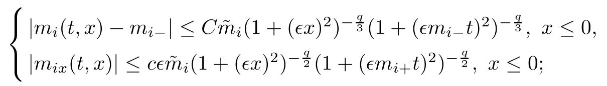
3 Proof of Theorem 1.1


4 A Priori Estimate


 Acta Mathematica Scientia(English Series)2020年5期