
EXISTENCE AND CONCENTRATION BEHAVIOR OF GROUND STATE SOLUTIONS FOR A CLASS OF GENERALIZED QUASILINEAR SCHRDINGER EQUATIONS IN RN?
2020-11-14 09:41:46JianhuaCHEN陳建華XianjiuHUANG黃先玖
Jianhua CHEN (陳建華) Xianjiu HUANG (黃先玖)?
Department of Mathematics, Nanchang University, Nanchang 330031, China
E-mail : cjh19881129@163.com; xjhuangxwen@163.com
Bitao CHENG (程畢陶)
School of Mathematics and Statistics, Qujing Normal University, Qujing 655011, China
E-mail : chengbitao2006@126.com
Xianhua TANG (唐先華)
School of Mathematics and Statistics, Central South University, Changsha 410083, China
E-mail : tangxh@mail.csu.edu.cn
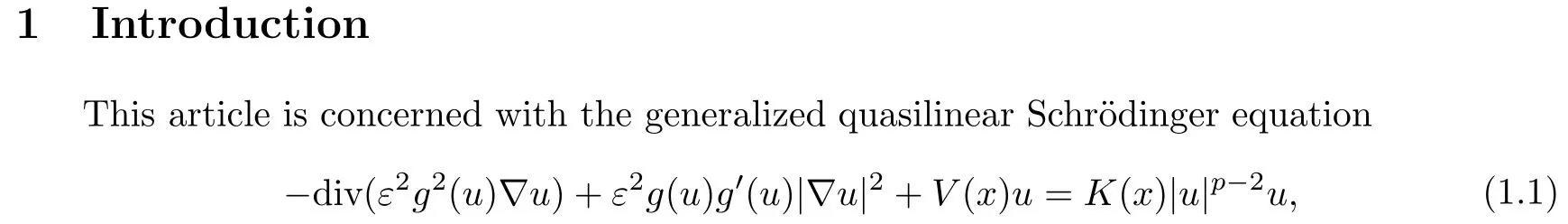
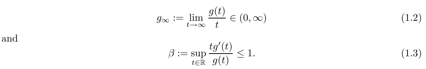
(g) g ∈ C1(R,(0,+∞)) is even with g′(t)≥ 0 for all t ∈ [0,+∞) and satisfies
It is well known that solutions of(1.1)are related to the existence of standing wave solutions for the following quasi-linear Schrdinger equation:

where z : R × RN→ C, W : RN→ R is a given potential, l : R → R and k : RN× R → R are suitable functions. For various types of l, the quasilinear equation of the form (1.4) has been derived from models of several physical systems. In particular, l(s) = s was used for the superfluid film [23, 26]equation in fluid mechanics by Kurihara [23]. For more physical background, we can refer to [4, 7, 22, 25, 36, 37, 39]and references therein. In fact, many conclusions about the equation (1.4) with l(t) = tαfor some α ≥ 1 have been studied; see[2, 27–29]and the references therein. However,to the best of our knowledge,only in the recent papers [16]and [46], the equation (1.4) with a general l were studied.
Setting z(t,x)=exp(?iEt)u(x),where E ∈ R and u is a real function,(1.4)can be reduced to the corresponding equation of elliptic type (see [30]):
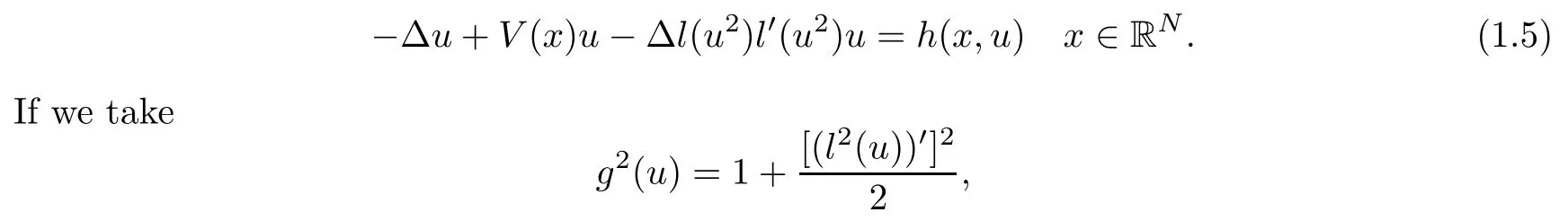
then (1.5) turns into the quasilinear elliptic equations ([46])

For(1.6),there are many papers(see[8–11,31,44–46])studying the existence of solutions.For example, in [15, 16], Deng et.al. proved the existence of positive solutions with critical exponents, where critical exponents are 2?and α2?, respectively. In [17, 18], Deng et.al.proved the existence of nodal solutions via the variational method. Very recently, in [32], Li et.al. proved the existence of ground state solutions and geometrically distinct solutions via the Nehari manifold method. In [33], the authors studied the existence of a positive solution,a negative solution, and infinitely many solutions via the symmetric mountain pass theorem.With regard to the generalized quasilinear Schrdinger equation of Kirchhoff type and the generalized quasilinear Schrdinger-Maxwell system, we can refer to [12, 13, 31, 51]and the references therein.
For the concentration behavior of solutions of (1.1), there is only one paper studying the equation

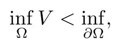
where N ≥3, and V(x) satisfies the following condition:

Under the above condition regarding the potential V(x), Li and Wu [34]studied the existence,multiplicity, and concentration of solutions by the Ljusternik-Schnirelmann theory.

For problem (1.9), with the local potential condition given by
where ? is a bound domain in RN, Wang and Zou[48]studied the existence and concentration of bounded state solutions with an (AR)-condition by the variational technique with N ≥3.Specifically, the authors first used the penalized nonlinearity developed by Pino and Felmer[38], and they worked on a suitable Orlicz space and established the asymptotic behavior of V as ε → 0. Finally, they proved the exponential decay phenomenon of bounded state solutions. For N = 2, doand Severo [19]proved the existence and concentration behavior of positive ground state solutions where ε>0 is a small positive parameter and allowing f(u) to enjoy critical exponential growth. They mainly used a version of Trudinger-Moser inequality,a penalization technique, and a mountain-pass argument in nonstandard Orlicz space. Afterwards, for problem (1.9) with potential condition (1.8), He, Qian and Zou [21]proved the existence and concentration of positive ground state solutions with an (AR)-condition by employing the Nehari manifold method, the mountain pass theorem and a compactness argument.More specifically,they employed an argument developed by Liu et.al. [28]to reformulate(1.9).They used some classical arguments developed by Brezis and Nirenberg [5]to prove that the corresponding energy functional satisfies the (PS)-condition, which plays an important role in applying the Ljusternik-Schnirelmann theory.
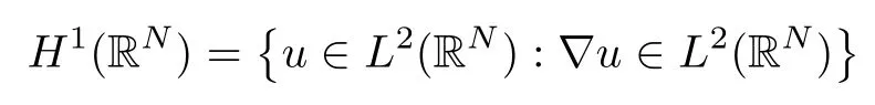
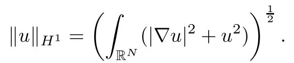
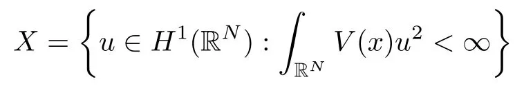
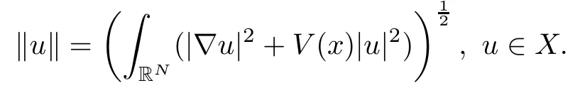
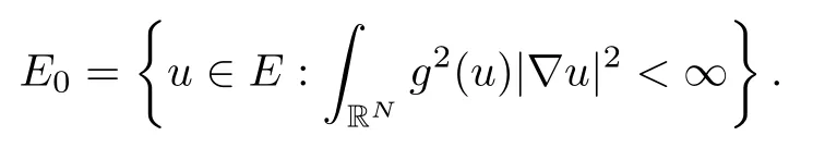
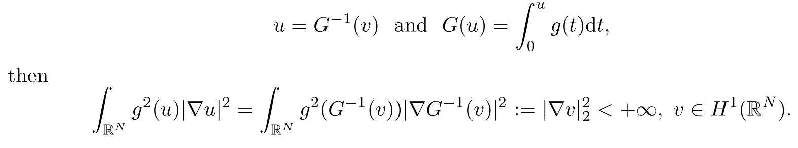
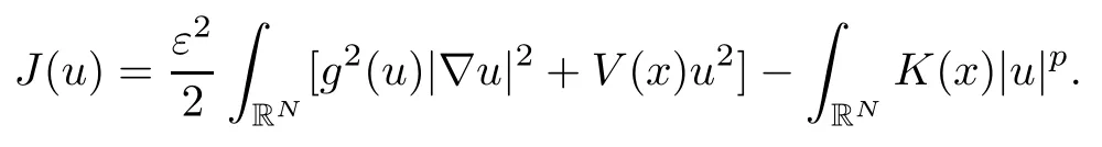
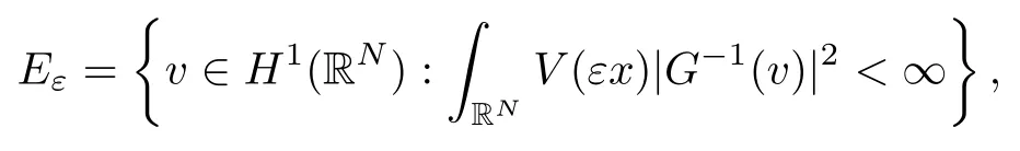
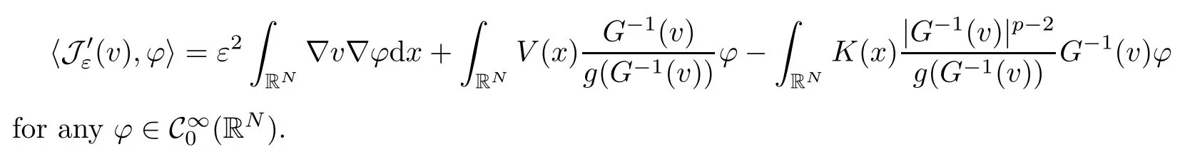
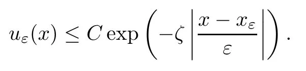
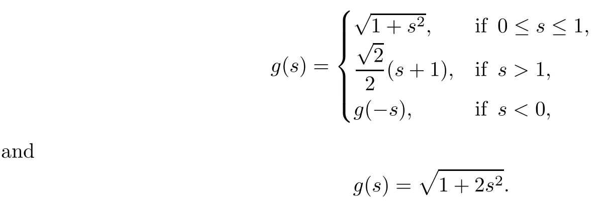
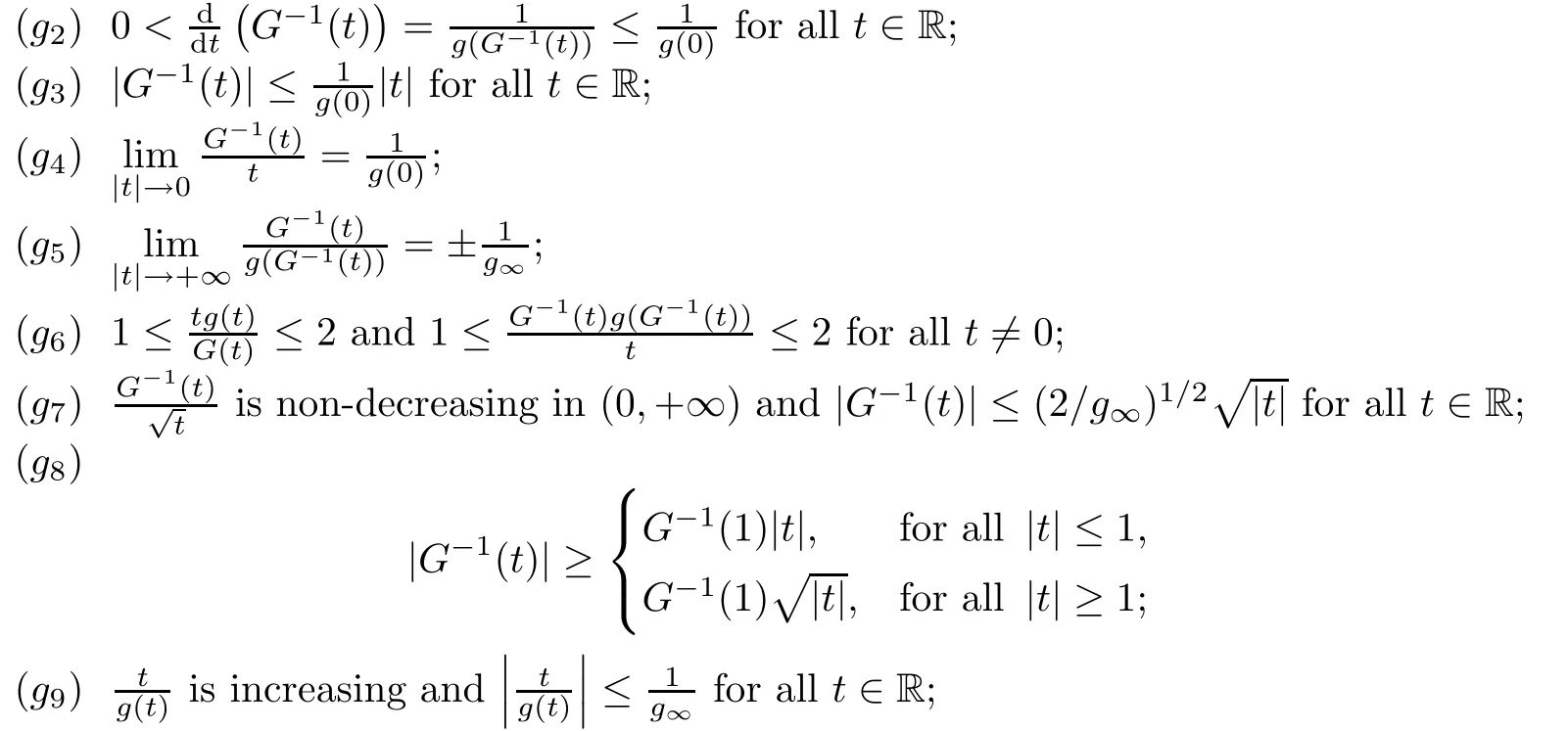
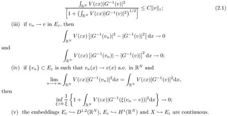
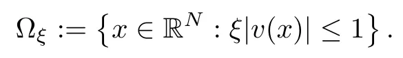
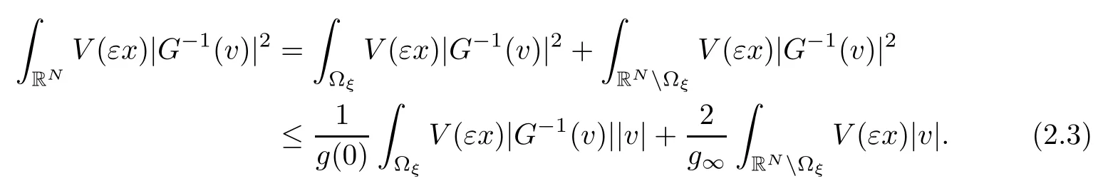
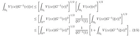
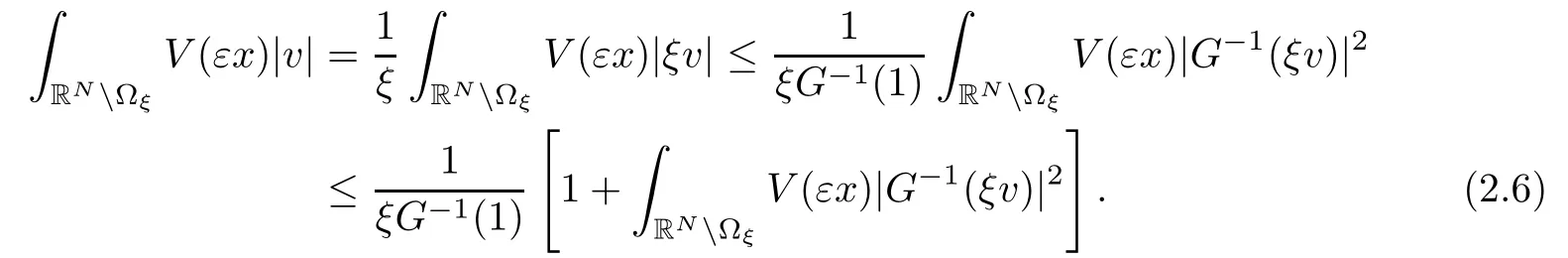
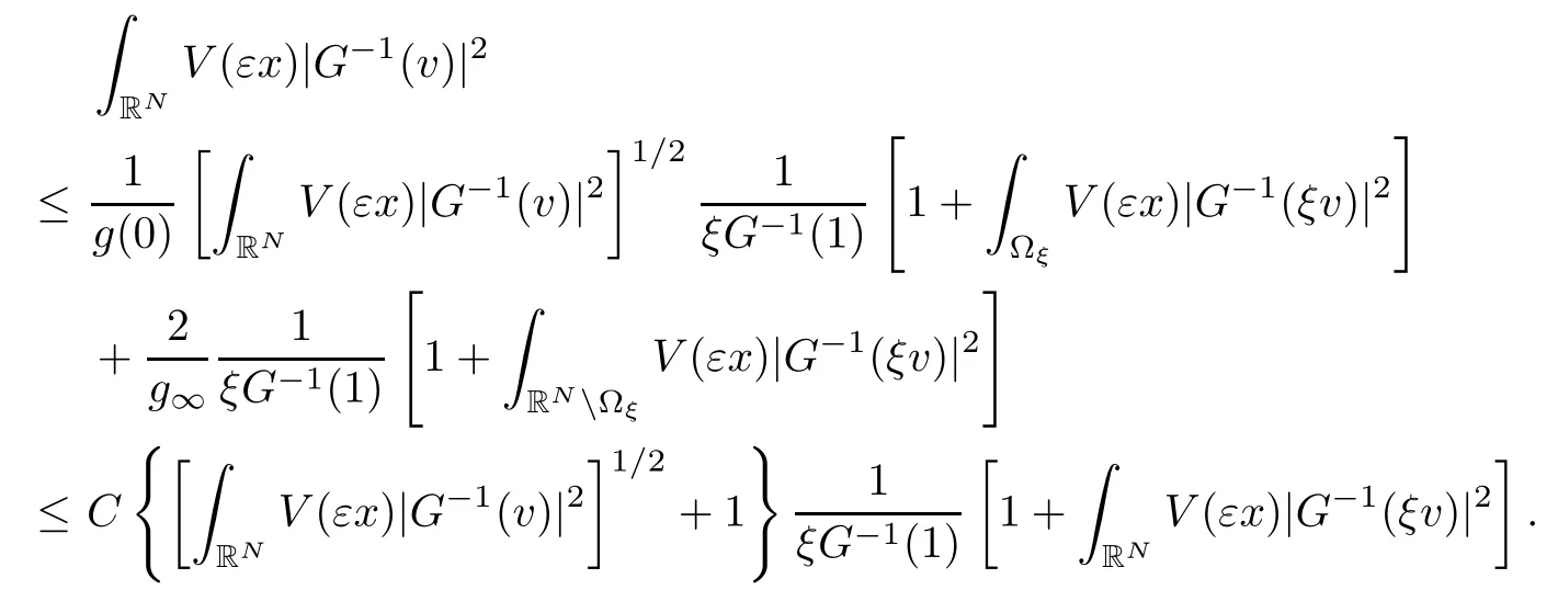
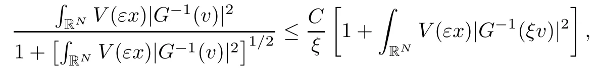
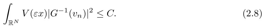
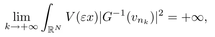
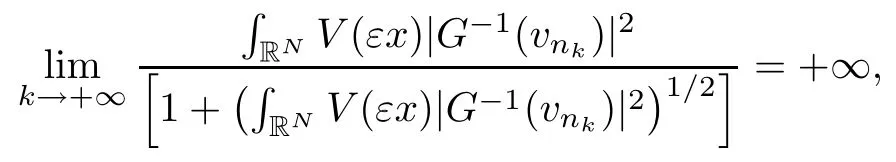
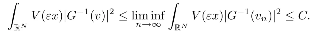
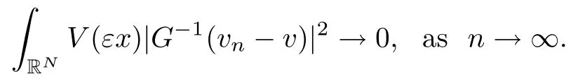
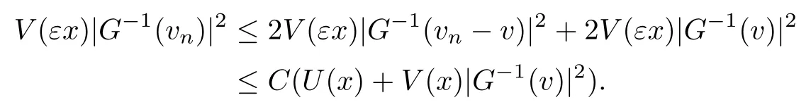
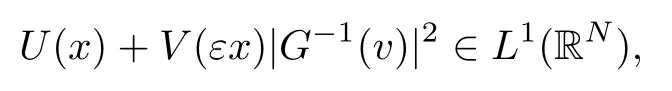
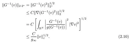
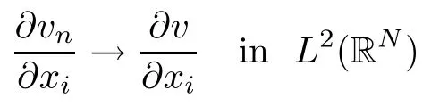
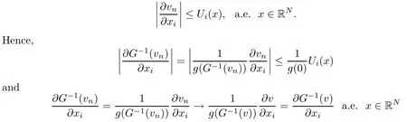
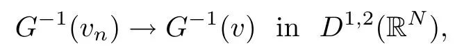
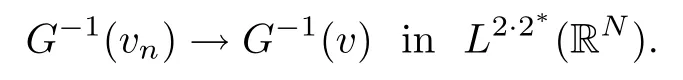
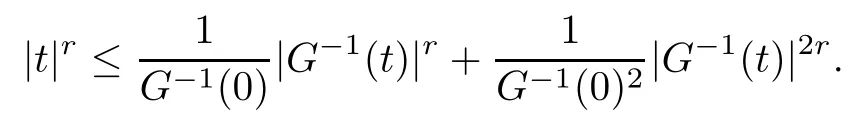
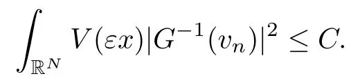
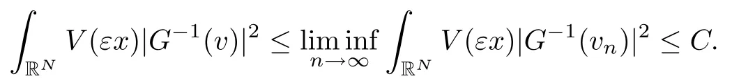
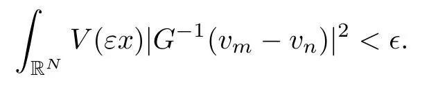
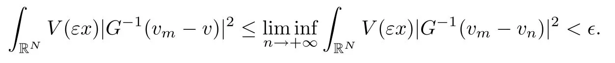
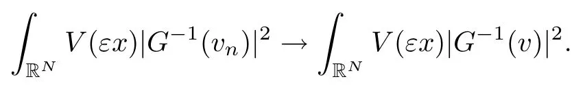
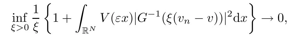
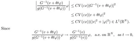
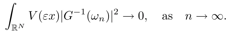
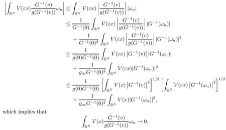
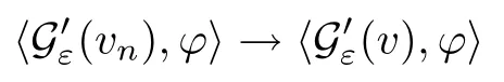
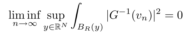
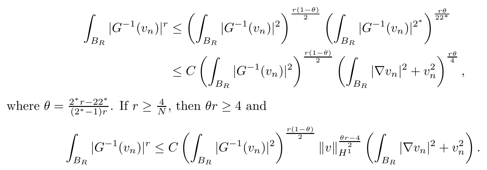
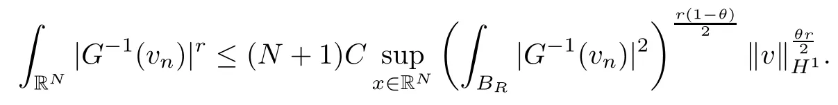
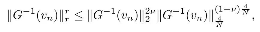
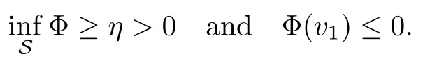
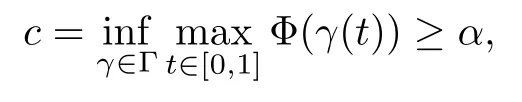
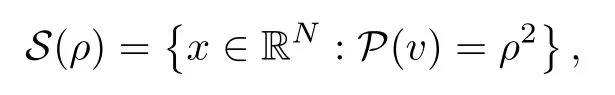
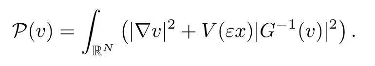
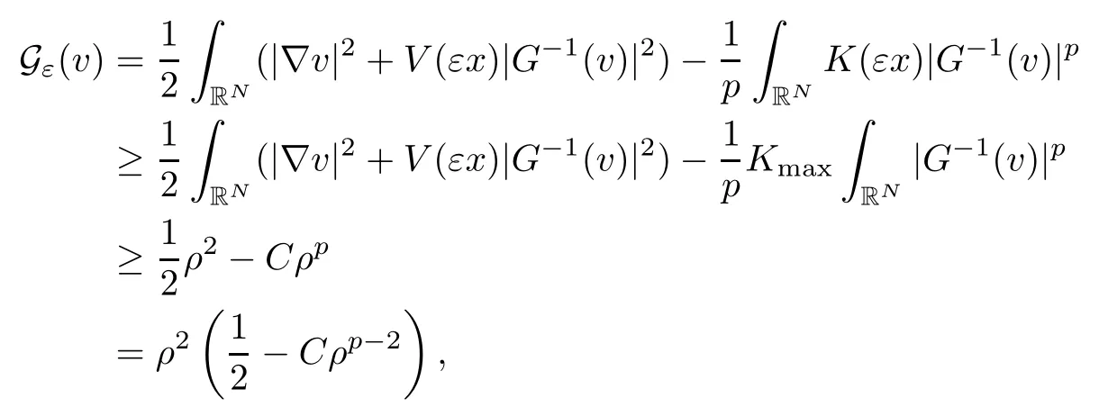
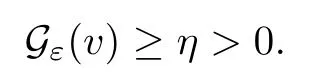
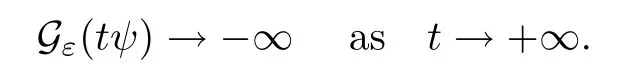
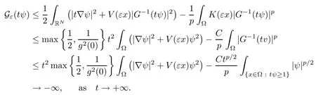
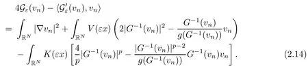
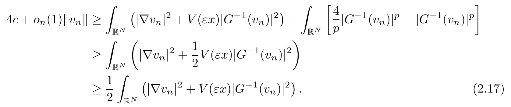
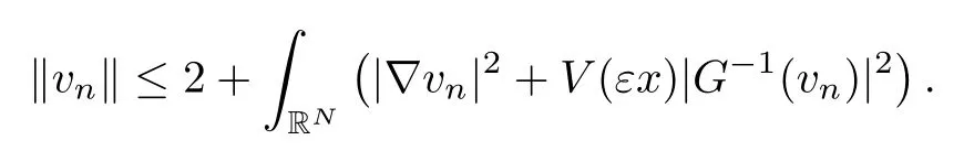
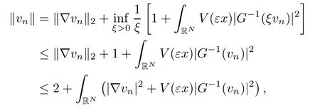
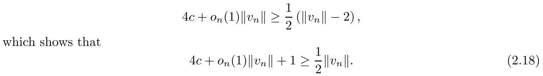
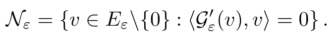
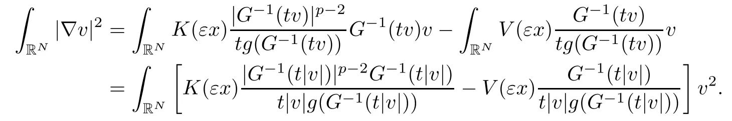
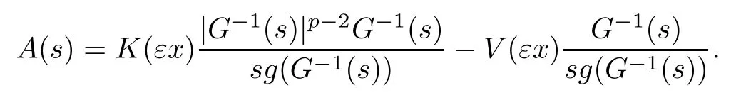
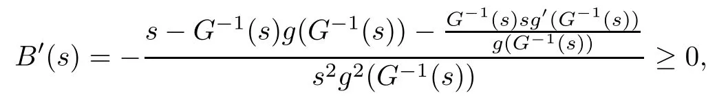
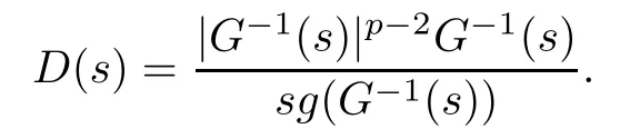
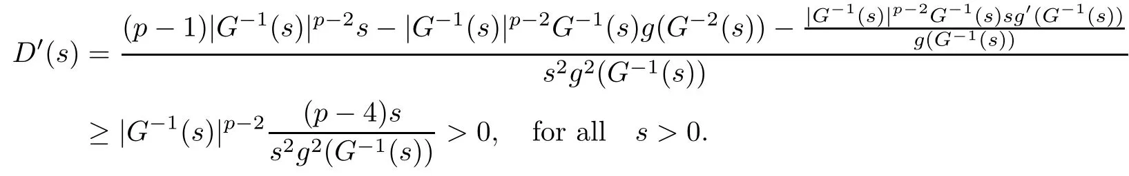
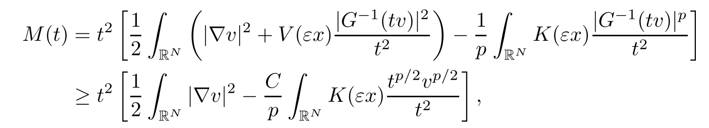
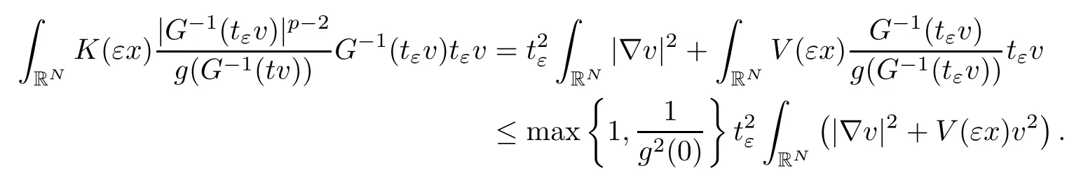
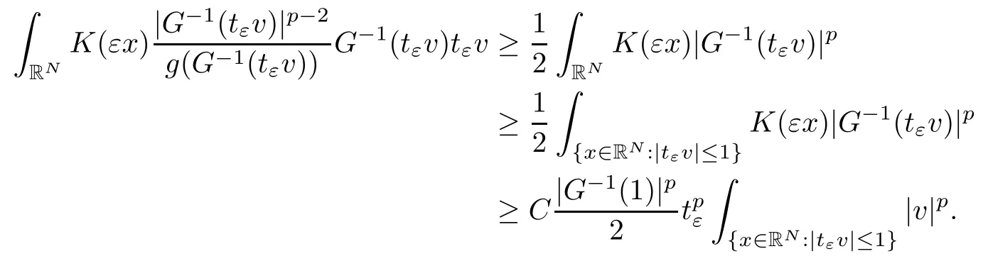
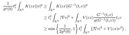
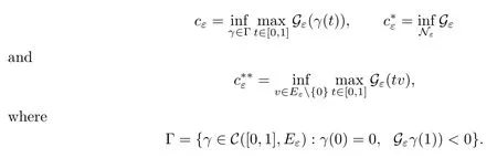
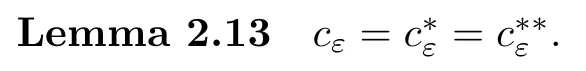
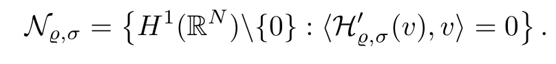
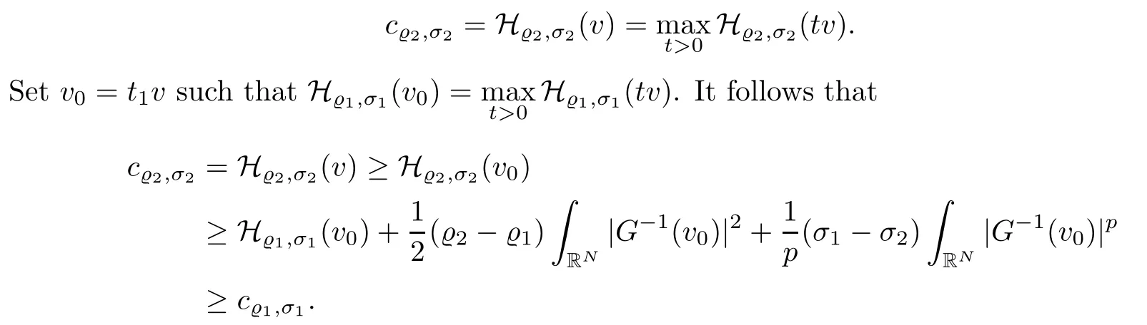
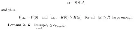
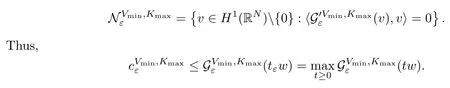
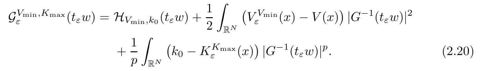
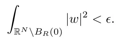
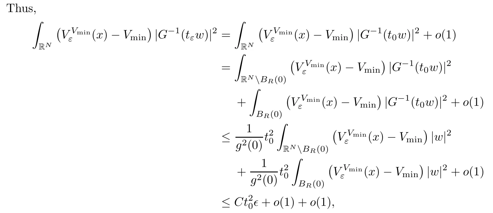
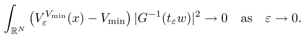
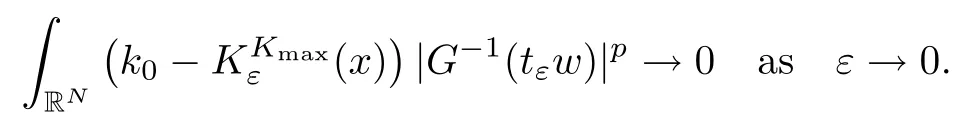
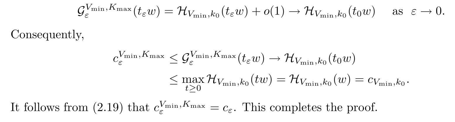
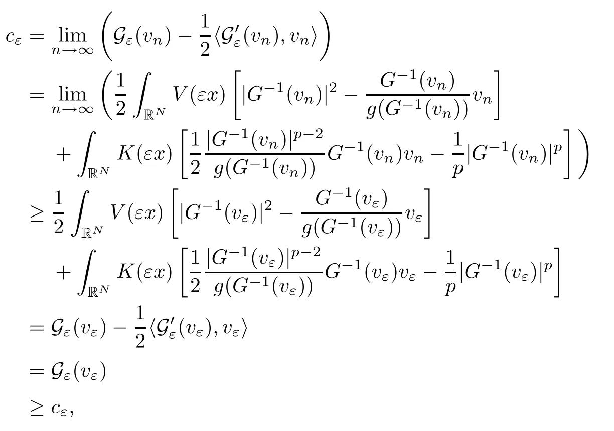
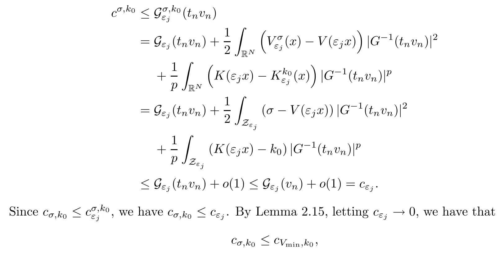
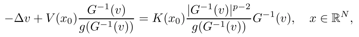
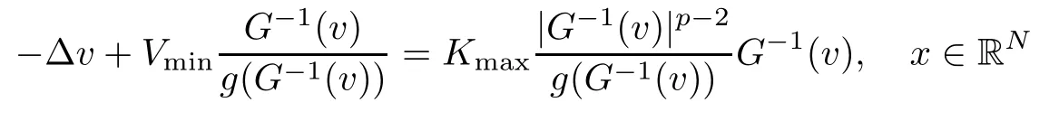
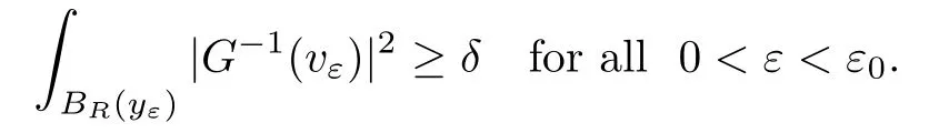
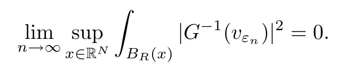
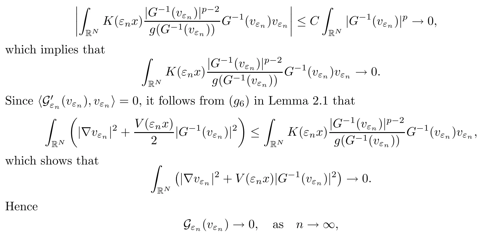
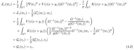
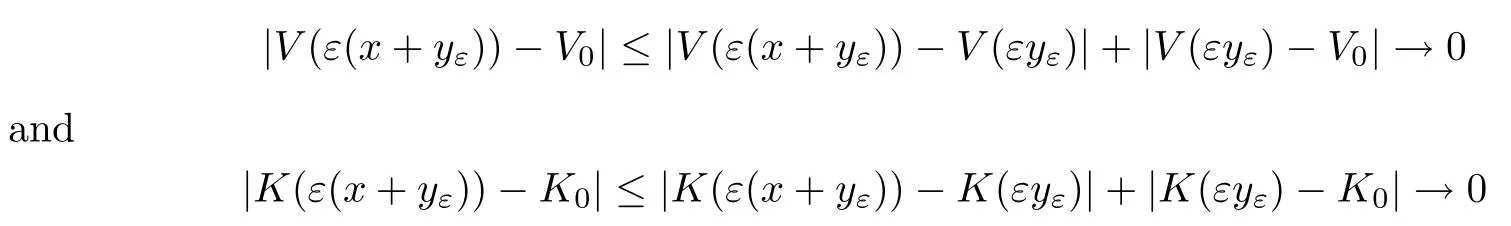
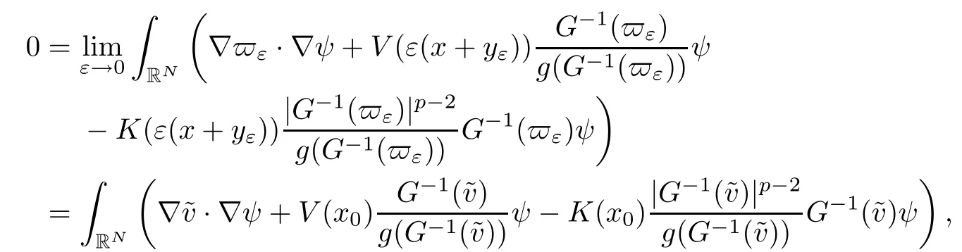
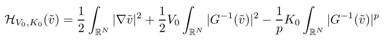
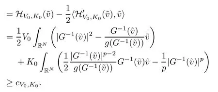
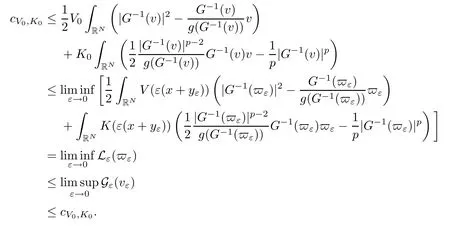
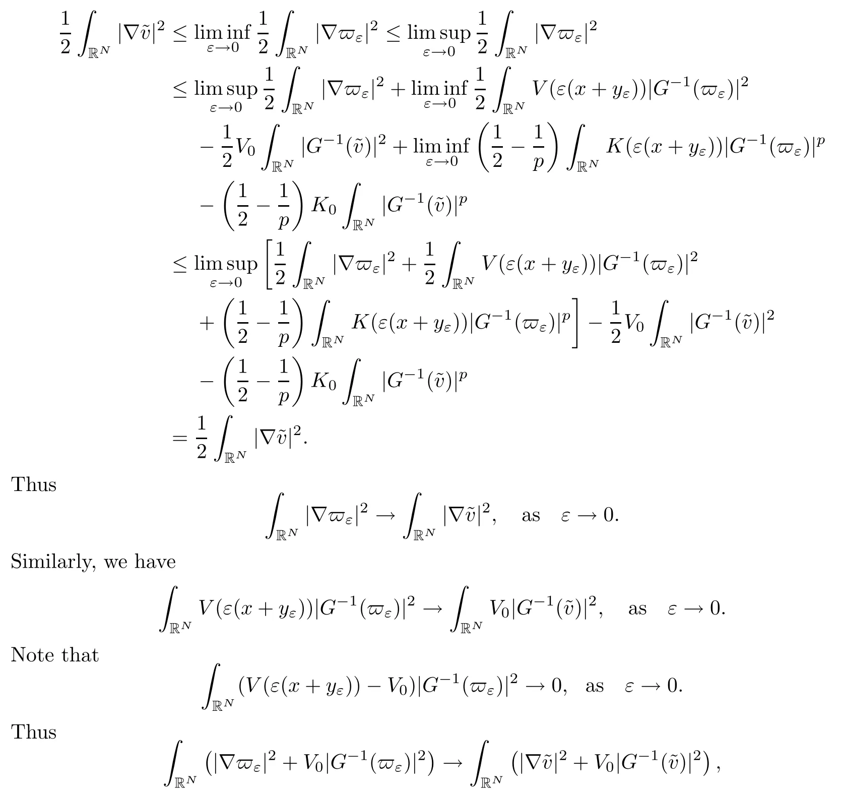
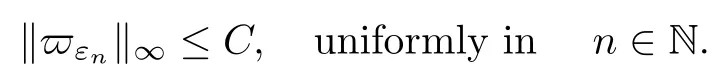
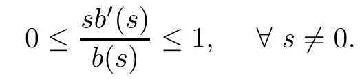
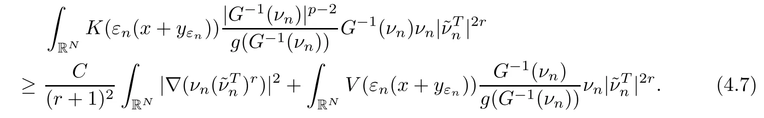
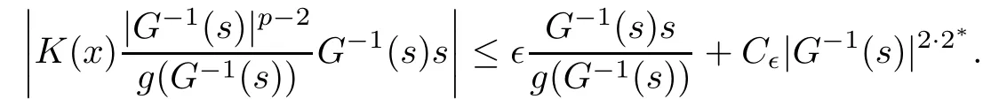
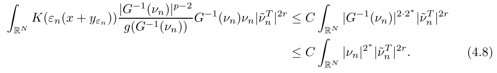
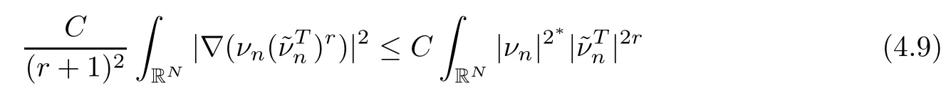
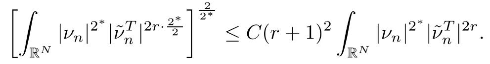
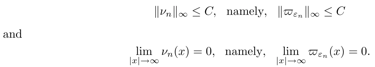
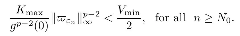
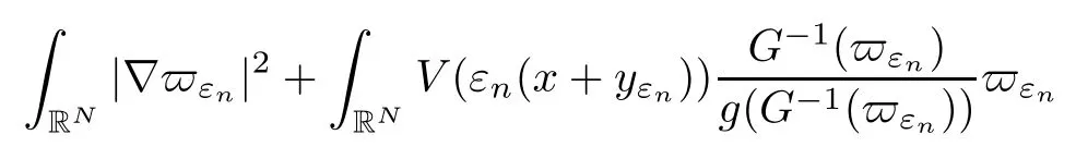
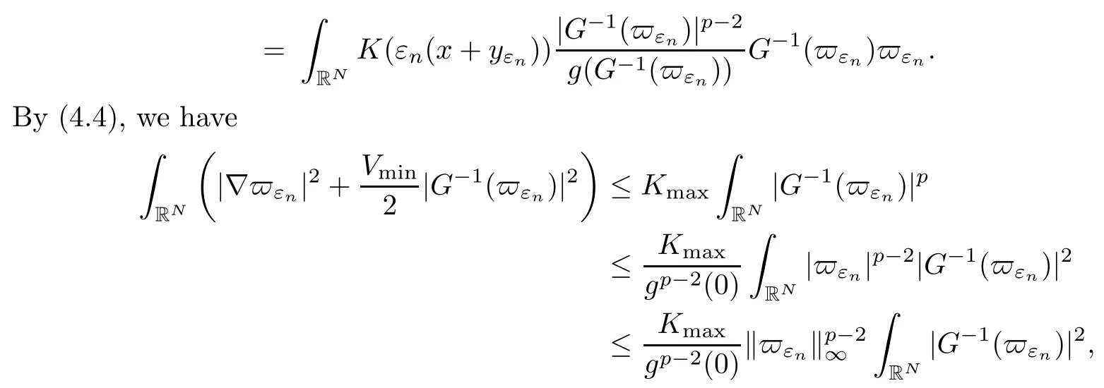
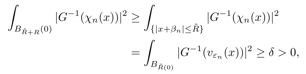
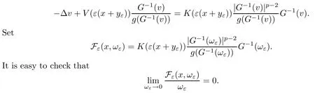
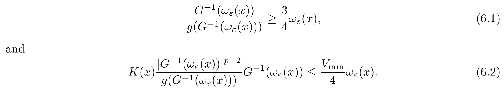
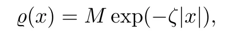
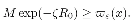
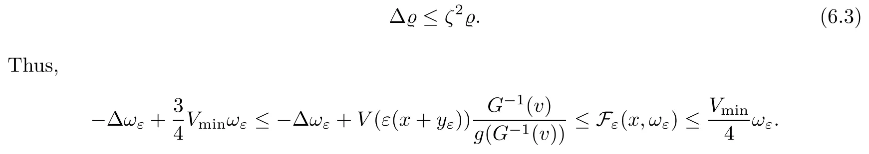
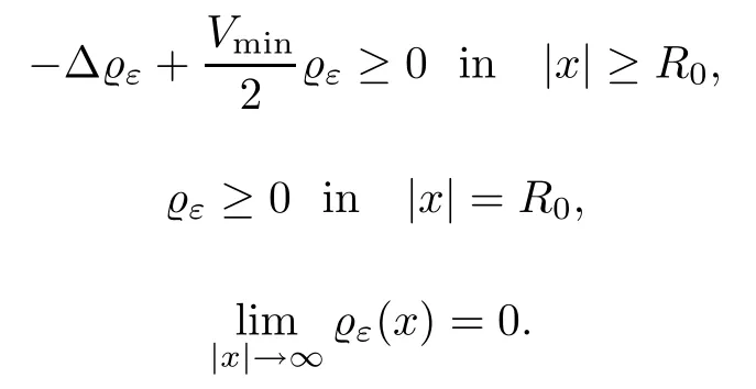
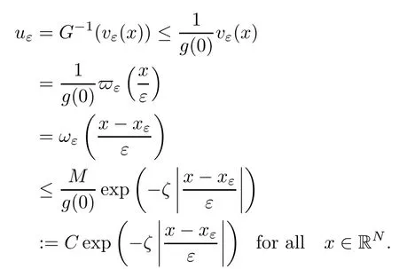
On the other hand, if f(u) = K(x)|u|p?2u in (1.9), there are many papers studying the existence and concentration of solutions. In [43], the authors assumed that V(x) and K(x) are uniformly continuous with V(x) possessing at least one minimum and K(x)having at least one maximum, where 4 A natural question is whether problem (1.1) has the existence and concentration behavior of positive ground states as ε → 0. To our knowledge,the existence and concentration behavior of the positive ground state solutions to eq. (1.1) have never been considered by variational methods except for in [34]. It is worth pointing out that there are many difficulties in treating this class of generalized quasilinear Schrdinger equation in RN. The most prominent difficulties that we need to overcome are: (I) the lack of compactness;(II) that the term ε2g(u)g′(u)|?u|2prevents us from working directly in a classical working space. In order to overcome the first difficulty, we use the concentration compactness lemma. To overcome the second difficulty,we give a new and suitable working space, that is, the Orlicz space which was given in [20].Moreover, motivated by [19], we will give some properties of the Orlicz space which are richer than those put forward in [20]. In this paper, we will give an affirmative answer to the question mooted above. First,however, we want to discuss some more properties of our working Orlicz space. Under the properties of this working space, we prove the existence of positive ground state solutions via the Nehari manifold method for enough small ε>0,and we establish the concentration behavior and the exponential decay phenomenon of ground state solutions as ε → 0. Before stating our results, we need to establish some properties of V and K: To state our results, we need to give the following assumptions on V and K: (VK1)V,K ∈ L∞(RN),V(x)and K(x)are uniformly continuous in RN, Vmin>0,inf K >0; (VK2)Vmin (VK3)K∞ By the condition (VK2), we can assume thatand let If (VK3) holds, we assume thatand let It is obvious that O1and O2are bounded sets. Moreover,ifthen O1=O2=A∩B. Now, let us recall some basic notions. Let with the norm It is well known that in the study of the elliptic equations, the potential function V plays an important role in the choosing of a right working space and some suitable compactness methods. General speaking, in order to study (1.1), the following working space is given: endowed with the norm To solve the equation (1.1), due to the appearance of the nonlocal termthe right working space seems to be It is easy,however,to see that E0is not a linear space under the assumption of(g). To overcome this difficulty, for any v ∈H1(RN), Shen and Wang [46]made the following change of variable: In such a case, we can deduce formally that the Euler-Lagrange functional associated with the equation (1.1) is In this paper, we want to define the following working space: which is called the Orlicz-Sobolev space. Eεis a Banach space (see [20]) endowed with the following norm: Furthermore, one can easily derive that if v ∈C2(RN) is a critical point of (1.12), then u=G?1(v)∈C2(RN) is a classical solution to the equation (1.1). By this change of variables,X can be used as the working space and (1.1) can be written as The energy functional of (1.11) is given by Moreover, we say that v ∈ Eεis a weak solution to the equation (1.11) if it holds that Since g is a nondecreasing positive function, we getFrom this and our hypotheses, it is clear that Jεis well defined in Eεand Jε∈ C1. Then it is standard to obtain that v ∈ Eεis a weak solution to the equation (1.11) if and only if v is a critical point of the functional Jεin Eε. To sum up,it is sufficient to find a critical point of the functional Jεin Eεto achieve a classical solution to the equation (1.1). Now, we state our first results by way of the following theorem: Theorem 1.1Suppose that (g), (VK1) and (VK2) hold. Then, for all small ε>0, (i) Equation (1.1) has a positive ground state solution uε; (ii) uεhas a global maximum point xεsuch that= 0 and xε→ x0as ε → 0, uε(εx+xε) converges in H1(RN) to a positive ground state solution of as ε → 0; (iii) there exist two constants ζ,C >0 such that Theorem 1.2If(g),(VK1)and(VK3)hold,and we replace O1by O2,then all conclusions of Theorem 1.1 are still true. Remark 1.3There are indeed functions which satisfy (g). Two examples are given by The paper is organized as follows: in Section 2, we give some preliminary lemmas. In Section 3, we will prove the existence of ground state solutions. In Section 4, we will establish the concentration behavior of ground state solutions. In Section 5, we will complete the proof of (i) and (ii) in Theorem 1.1. In Section 6, we give an exponential decay of these solutions. NotationsThroughout this paper, we make use of the following notations: ? Lr(RN) denotes the Lebesgue space with norm ? for any z ∈ RNand R>0, BR(z):={x ∈ RN:|x ? z| ? the weak convergence in H1(RN) is denoted by ?, and the strong convergence by →; ? exp(·) denotes the exponential functions; In this section, motivated by [19], we present some useful lemmas and corollaries. Now, let us recall the following lemma which has been proved in [20]: Lemma 2.1(see [20]) For the functions g, G, and G?1, the following properties hold: (g1) the functions G(·) and G?1(·) are strictly increasing and odd; (g10) the function [G?1(t)]2is convex. In particular,[G?1(θt)]2≤ θ[G?1(t)]2for all t ∈ R,θ ∈ [0,1]; (g11) [G?1(θt)]2≤ θ2[G?1(t)]2for all t ∈ R, θ ≥ 1; (g12) [G?1(t1?t2)]2≤ 4([G?1(t1)]2+[G?1(t2)]2) for all t1,t2∈ R; (g13) the function G?1(t) is concave. In particular, G?1(θt) ≤ θG?1(t) for all t ∈ R,θ ∈ [1,+∞); (g14) G?1(θt)≥ θG?1(t) for all t ∈ R, θ ∈ [0,1]. Lemma 2.2The space Eεhas the following properties (i) Eεis a normed linear space with respect to the norm given in (1.10); (ii) there exists a positive constant C >0 such that for all v ∈ Eε, ProofBy (g11) in Lemma 2.1, we have First, we can clearly observe that 0 ∈ Eε. Secondly,let v ∈ Eε, α ∈ R{0}and k ∈ N such that|α|/2k∈ (0,1). By (g10) in Lemma 2.1, (2.2), and using that G?1(v) is convex, we have and thus αv ∈ Eε. Let v1,v2∈ Eε, and using that G?1(v) is convex again, we obtain Thus Eεis a linear space. It is standard to prove that (1.10) is a norm in Eε(see [20]). Next, we give a proof of (ii). Now, for any v ∈ Eεand ξ >0, set From (g3) and (g7) in Lemma 2.1, we have To prove (ii), it is easy to check the following elementary inequality: On the one hand, by (2.4), Hlder inequality and (g8) in Lemma 2.1, we have On the other hand, using (g8) in Lemma 2.1 and (2.4), we have Hence from (2.3), (2.5) and (2.6), we can infer that for all ξ >0, Thus, for all ξ >0, one has which implies that Next, we prove (iii). By (2.4), we get the following limit: Thus, from (2.7) and (2.1), we have In fact, if we suppose to the contrary that there exists a subsequence {vnk}? Eεsuch that then by (2.7), we can infer that which contradicts (2.1). Thus, (2.8) holds. Since vn→ v in Eε, one has that By (2.1), we have that By Lemma A.1 in [49], up to a subsequence, there exists U ∈L1(RN) such that Hence, by (2.2), together with the convexity of G?1(v), we have Since by the Lebesgue dominated convergence theorem, we can finish the proof of (iii). For (iv) and(v), the proof is given in [20]when N ≥3. We omit the proof. Lemma 2.3The mapfrom Eεto Lr(RN)is continuous for each r ∈ [2,2·2?]. ProofLet v ∈ Eε. By definition, we know that G?1(v) ∈ X, which, together with Lemma 2.2 and (g2) in Lemma 2.1, implies that for all 2 ≤ r ≤ 2?. Moreover,by the Gagliardo-Nirenberg inequality and(g9)in Lemma 2.1,we have Thus, for all v ∈ Eε, we know that G?1(v) ∈ L2·2?(RN). Let {vn} be a sequence in Eεsuch that vn→ v in Eε. Thus for i=1,2,··· ,N. By (iii) in Lemma 2.2, we have Therefore, by Lemma A.1 in [49], up to a subsequence, there exists Ui∈L2(RN) for i =1,2,··· ,N such that for i=1,2,··· ,N. Thus, by the Lebesgue dominated convergence theorem, we have which, together with (2.11), gives Moreover, by Lemma 2.2-(v), one has By (2.10), we have Again, by Lemma A.1 in [49], there exists W ∈ L2?(RN) such that By the convexity of G?1(v)2, we get Hence, by the Lebesgue dominated convergence theorem, one has that This complete the proof. Lemma 2.4The embeddingis continuous for 2 ≤ r ≤ 2?. ProofFirst, by (g8) in Lemma 2.1, we can get that Moreover,if v ∈ Eε, then v ∈ Lq(RN) for 2 ≤ q ≤ 2?. By Lemma 2.3, if vn→ 0 in Eε, then we have G?1(vn)→ 0 in Lq(RN) for 2 ≤ q ≤ 2?. Using (2.12), we have It follows that vn→ 0 in Lr(RN) for 2 ≤ r ≤ 2?. Thus the result obviously holds. Proposition 2.5Eεis a Banach space. Moreover,is dense in Eε. ProofWe want to prove the first part in this proposition. Suppose that{vn}is a Cauchy sequence in Eε. By (v) in Lemma 2.2, we know that {vn} is a Cauchy sequence in D1,2(RN).Using the completeness of the space D1,2(RN), there exists v ∈ D1,2(RN) such that vn→ v in D1,2(RN) and vn(x) → v(x) a.e. in RN. Thus {vn} is bounded in Eε. By (2.1), we have that there exists C >0 such that Moreover, by Fatou’s Lemma, we have Since 2·2?> 4, it follows from Lemma 2.3 that |G?1(vn)|2and |G?1(vn)|4are bounded in L1(RN). By (2.12), we obtain Thus v ∈ L2(RN), and consequently, v ∈ Eε. By (2.1), for any ?>0, there exists N0∈ N such that for all n,m ≥ N0, Fixing m>N0and applying Fatou’s lemma, we have By a similar argument as to that in the proof of property (iii) in Lemma 2.2, we can conclude that By (iv) in Lemma 2.2, we deduce that and consequently, vn→ v in Eε. In (1.11), we make the change of the variableso we can rewrite the equation(1.1)as follows: If v is a solution of the equation(2.13),then w(x):=v(x/ε)is a solution of the equation(1.11). Thus we only need to study the problem (2.13). Therefore, the energy functional is given by Proposition 2.6The functional Gεis well defined,continuous and Gateaux-differentiable in Eεwith Moreover,for v ∈Eε, we know thatand if vn→v in Eεthen for each ? ∈Eε; that is,in the weak ?topology of ProofIt is easy to check that Gε(v) is well defined. If vn→ v in Eε, then by (v) of Lemma 2.2, Moreover, by (iii) in Lemma 2.2, we have Thus Gεis continuous. Next, we prove that Gεis Gateaux-differentiable in Eε. Note that for any fixed v,? ∈ Eε,by the mean value theorem there exists 0<θ <1 such that For any |t|≤1, we have by the Lebesgue dominated convergence theorem we have Similarly, we can conclude that Based on the above discussion, we know that Gε∈ C1(Eε,R). Moreover, it follows from (g2), (g9) in Lemma 2.1 and (2.12) that In a fashion similar to the proof of the first part of this proposition, we can prove that if vn→ v in Eε, then Next, we want to give an important lemma named the vanishing Lemma. Lemma 2.7Let {vn} be a bounded sequence in Eεsuch that for some R>0. Then G?1(vn)→ 0 in Lr(RN) for 2 ProofAsis continuous, in a fashion similar to the proof of Lemma 2.2 in [48], we know that {vn} is a bounded sequence in H1(RN). It follows from the Hlder and Sobolev inequalities that Covering RNby a family of balls {BR(yi)} such that each point is contained in at most N +1 such balls and summing up these inequalities over this family of balls, we obtain and the result in this case follows the conclusion already established above. The next two lemmas show that the functional Gεverifies the mountain pass geometry.Before proving the two lemmas,we need to the following version of the mountain pass theorem,which is a consequence of the Ekeland variational principle as developed in [1]: Theorem 2.8(see [1]) Let Eεbe a Banach space and Φ ∈ C(Eε,R) be Gateauxdifferentiable for all v ∈Eε, with G-derivative Φ′(v) ∈continuous from the norm topology of Eεto the weak ?topology of, and Φ satisfying the (PS) condition and Φ(0)= 0. Let S be a closed subset of Eεwhich disconnects (archwise) Eε. Let v0= 0 and v1∈ Eεbe points belonging to distinct connected components of EεS. Suppose that Then and there exists a (PS)csequence for Φ. Hence, c is a critical value of Φ. Next, we prove that Gεsatisfies all the conditions of Theorem 2.8. To this end, for ρ > 0,let us define the following set: where P :Eε→ R is given by Because P(v) is continuous, S(ρ) is a closed subset and disconnects the space Eεfor ρ >0. Lemma 2.9There exist η,ρ >0 such that Gε(v)≥ η for all v ∈ S(ρ). ProofBy (v) of Lemma 2.2, for v ∈ Sρ, we get This completes the proof. Lemma 2.10There exists v ∈ Eεsuch that P(v)> ρ2and Gε(v)<0. ProofTo this end, we only need to show that for any ψ ∈ Eε{0}, This completes the proof. Lemma 2.11Any (PS)csequence for Gεis bounded in Eε. ProofSuppose that {vn} is a (PS)cfor Gε, that is, Gε(v) →c and→0. Using(g), Using the definition of G, we can get G(t) ≤ g(t)t for all t ≥ 0. In fact, by g′(t) ≥ 0 for all t ≥0, By (2.15) and (g6) in Lemma 2.1, it is easy to check that By (2.14) and (2.16), we have Next, we prove In fact, by the definition ofand s1/2≤ 1+s for all s ≥ 0, we have which shows that the inequality holds. Thus, by (2.10) and (2.17), we have that It follows from (2.18) that {vn} is bounded in Eε. Next, to characterize the least energy of Gε, we define the following Nehari manifold: Thus, for any v ∈ Nε, we know that Now, we prove an important lemma for the energy functional Gεas follows: Lemma 2.12For any v ∈ Eε{0}, there exists a unique tε> 0 such that tεv ∈ Nε.Moreover, Gε(tεv) = maxt≥0Gε(tv). Moreover, there exist T1> T2> 0 independent of ε > 0 such that T2≤ tε≤ T1. ProofFirst, we prove the first part of this lemma. For t>0, we define Note that the right hand of the equality is an increasing function on t > 0. In fact, for any fixed x ∈ RN, we consider a function A:(0,∞)→ R given by Then, by (g) and (g6) in Lemma 2.1, one has This shows that D(s) is increasing in (0,+∞). By these two facts, we have that A(s) is increasing in (0,+∞). It follows that which implies that M(t)>0 for t>0 small. Moreover,M(0)=0,and by the above inequality,we know that M(t) = Gε(tv) < 0 for t > 0 large. Therefore, by the monotony of A(s), we have that there exists a unique tε> 0 such that M′(tε) = 0; that is, tεv ∈ N. Furthermore,M(tε)= Now, we prove the second part of this lemma. Since tεv ∈ Nε, by (g6) in Lemma 2.1 we have Moreover,by (g6) in Lemma 2.1, one has Thus there exists T1>0 independent of ε such that tε≤ T1. On the other hand, by (g6) in Lemma 2.1, we have which implies that there exists T2>0 independent of ε such that tε≥ T2. This completes the proof. In order to obtain a ground state solution, we need a characterization of the least energy.We consider the following: By a standard argument (see [14, 40, 49, 50]), we can get the following lemma: Next, we consider the autonomous problem and the corresponding energy functional In a fashion similar to the proof of Lemma 2.9–2.11, it is easy to check that Hpossesses the mountain pass structure, and hence that Hhas a bounded (PS)-sequence, and its least energy has the same characterization as stated in Lemma 2.13. Using the fact that His invariant under translation, we know thatis attained, where cis the Mountain Pass level value and Nis given by Lemma 2.14Letj> 0 and σj> 0, j = 1,2, with1≤2and σ1≥ σ2. Then c≤ c. In particular, if one of the above inequalities is strict, then c ProofLet v ∈ Nbe such that This completes the proof. By the condition (VK2), without loss of generality, up to a translation, we may assume that ProofSet Vι(x)=max{ι,V(x)}, Kκ(x)=min{κ,K(x)},Kκ(εx), where ι,κ are positive constants. Define the energy functional for any v ∈H1(RN), which shows thatand thusis the least energy ofBy the definitions of Vminand Kmax, we get thatTherefore we have It follows that By Lemma 2.12,we can assume that tε→ t0as ε → 0. Since w ∈ L2(RN), for any ?>0, there exists R>0 such that Similarly, we know that Thus, by (2.20), one has that In this section, we will prove the existence of positive ground state solutions. Lemma 3.1cεis attained at some positive vε∈ Eε, for small ε>0. ProofBy Theorem 2.8,we know that Gεpossesses a(PS)cε-sequence in Eε,which means that there exists a sequence {vn}? Eεsuch that From Lemma 2.11, we know that {vn} is bounded in Eε, sinceis continuous.Thus {vn} is bounded in H1(RN). Up to a subsequence, there exists v0∈H1(RN) such that vn? vεin H1(RN), vn→ vεinfor 2 ≤ r ≤ 2?, vn(x) → vε(x) a.e. in RN. In a manner similar to the proof in [42], and by (3.1), we have that=0. Moreover,vε∈Eε.Thus, vεis a weak solution of (1.11). Ifthen vε∈ Nε. It follows from Lemma 2.1 and Fatou’s lemma that which is due to the fact that 4 From (VK1), we choose σ ∈(Vmin,V∞) and consider the energy functionalLetBy Lemma 2.12, we know that {tn} is bounded. Thus we assume that there exists t0such that tn→ t0as n → ∞. By (VK1) again, we can infer thator Kε(x)≥ k0} is bounded. Moreover,Gεj(tnvn)≤ Gεj(vn). Thus we have which is in contradiction to cVmin,k0 In this section, we will prove the convergence property of the ground state solution vεas ε → 0. Next, we commence by stating the following theorem: Theorem 4.1If vεis a solution of(1.11)given by Lemma 3.1,then vεpossesses a global maximum point yεsuch that, up to a subsequence, εyε→ x0as ε → 0,= 0 and vε(x+yε) converges in H1(RN) to a positive ground state solution of the equation as ε → 0. Next, we divide the proof of Theorem 4.1 into several steps. Lemma 4.2There exists a family {yε}0<ε<ε0in RNand there exist positive constants R>0 and δ >0 such that ProofSuppose, to the contrary,that there exists a sequence εn→ 0 as n → ∞ such that for all R>0, By Lemma 2.7, we conclude that G?1(vεn)→ 0 in Lr(RN)for all 2 which is in contradiction to Gεn(vεn)→ cεn>0. This completes the proof. with the energy functional Moreover, by virtue of V,K ∈ L∞(RN), without loss of generality, we may assume that V(εyε)→ V0and K(εyε)→ K0as ε → 0. Lemma 4.3is a positive ground state solution of ProofBy the continuity of V,K, we have that are uniformly on bounded sets of x ∈ RN. Then when ε → 0, one has that are uniformly on bounded sets of x ∈ RN. Thus V(ε(x+yε))→ V0and K(ε(x+yε))→ K0as ε → 0 are uniformly on bounded sets of x ∈ RN. By(4.1)and Lesbegue dominated convergence theorem, for anywe have By (g6) in Lemma 2.1, for any t ∈R, we have that From (4.4), (4.2), Fatou’s lemma and the proof of Lemma 2.15, we know that Hence, Lemma 4.4{εyε} is bounded. ProofSuppose, to the contrary,that passing to a subsequence, |εyε|→ ∞. Since V,K ∈L∞(RN), without loss of generality, we may assume that V(εyε) → V0and K(εyε) → K0as ε → 0. Moreover, by V(0) = Vminand k0= K(0) ≥ K(x) for all |x| ≥ R, we infer that V0>Vminand K0≤k0. Thus it follows from Lemma 2.14 that cV0,K0>cVmin,k0. By (4.5) and Lemma 2.15, cε→ cV0,K0≤ cVmin,k0, which is a contradiction. This completes the proof. Next, we need to assume that εyε→ x0as ε → 0. If we do so, then V0= V(x0) and K0=K(x0). ProofIn order to prove this conclusion, we only need to prove x0∈O1. Suppose the contrary; that is, thatBy (VK1) and Lemma 2.14, we have cV(x0),K(x0)> cVmin,k0.Thus it follows from Lemma 2.15 that which is a contradiction. This completes the proof. ProofBecauseis a ground state solution of (4.3), we have Lemma 4.7Let εn→ 0 andεnbe a solution of where yεnis given in Lemma 4.2. Thenand there exists a constant C > 0 such that ProofLet νn:=εn. In a manner similar to the method of [34], let T > 2, r > 0 andwhere b : R →R is a smooth function satisfying that: b(s) = s for |s| ≤T ?1,b(?s)=?b(s);b′(s)=0 for s ≥T and b′(s)is decreasing in[T ?1,T]. This shows thatforfor0 for |νn| ≥T,where T ? 1 ≤ CT≤ T. By the definition of b(s), we have By Lemma 2.1, for any ?>0, there exists C?>0 such that Moreover, by (g7) in Lemma 2.1 and the above inequality, we have By (4.7) and (4.8), we have From Sobolev inequality, we know that Combining this with (4.9) and (4.10), one has that Next, the proof is the same as that of Lemma 4.6 in [24, 34]. It is easy to check that there exists C >0 such that This completes the proof. Lemma 4.8There exists α >0 such thatfor all n ∈ N. ProofAssume thatas n → ∞. For a giventhere exists N0∈N such that Thus one has In this section, we give the proof of our main results. Proof of Theorem 1.1Let βnbe the global maximum of. By Lemma 4.7 and Lemma 4.8, we have that βn∈ BR(0) for some R > 0. Hence the global maximum point vεnis given by βn+yεn. Define χn(x) := vεn(x+ βn+yεn), whereSince{βn} ? BR(0) is bounded, {εn(βn+yεn)} is bounded and εn(βn+yεn)→ x0∈ O1. It follows from the boundedness of {vεn} that {χn} is bounded in H1(RN). Assuming that χn? χ in H1(RN), χn? χ infor r ∈ [1,2?). Moreover, by Lemma 4.2, we have Next, In a fashion similar to the argument above,we can conclude that χ is a ground state solution of (4.3) and χn? χ in H1(RN). Therefore, χnpossesses the same properties as,and we can assume that yεnis a global maximum point vεn. Thus, by Lemma 4.2–4.6,we can get (i) and (ii) of Theorem 1.1, that is, this completes the proof of Theorem 4.1. In this section,we give an exponential decay of solutions. Let ωεbe a ground state solution of the following equation: Thus we can choose R0>0 such that for all |x|≥R0, Now, we define where ζ and M are such that 4ζ2 It is easy to check that, for all By the maximum principle, we know thatε(x)≥ 0 for all |x|≥ R0. Hence, which implies that This completes the proof of (iii) in Theorem 1.1. The argument for Theorem 1.2 is similar to that for Theorem 1.1, so we omit it.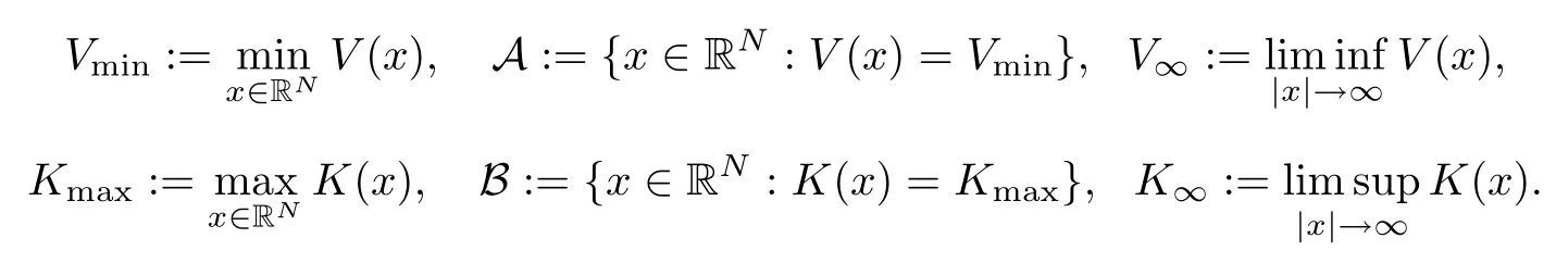


2 Some Preliminary Lemmas


3 Existence of Ground State Solutions

4 Concentration and Convergence of Ground State Solutions


5 Proof of Theorem 1.1
6 The Exponential Decay of Solutions

 Acta Mathematica Scientia(English Series)2020年5期