BAI Hong-fang, XU Rui

(1.Faculty of Science and Technology, University of Macau, Macau Special Administrative Region,China; 2.Complex Systems Research Center, Shanxi University, Taiyuan, 030006, China)

Abstract: In this paper, an eco-epidemiological model with Beddington-DeAngelis functional response and a time delay representing the gestation period of the predator is studied.By means of Lyapunov functionals and Laselle’s invariance principle,sufficient conditions are obtained for the global stability of the interior equilibrium and the disease-free equilibrium of the system, respectively.

Key words:Eco-epidemiological model;delay;Laselle’s invariance principle;global stability

§1. Introduction

It is necessary to study the effect of epidemiological parameters in the ecological domain from mathematical as well as ecological point of view. As a new branch in mathematical biology, eco-epidemiology merges ecology and epidemiology to understand the dynamics of disease propagation on the prey-predator population.

The disease factor in predator-prey system was first introduced by Anderson and May [1].Since this pioneering work, great attention has been paid to the modeling and analysis of eco-epidemiological systems recently, and an increasing number of works have been devoted to the study of the relationships between demographic processes among different populations and diseases [2-12]. Such as, Zhang et al. [8]studied the following delayed eco-epidemiological model with Holling type-I response function

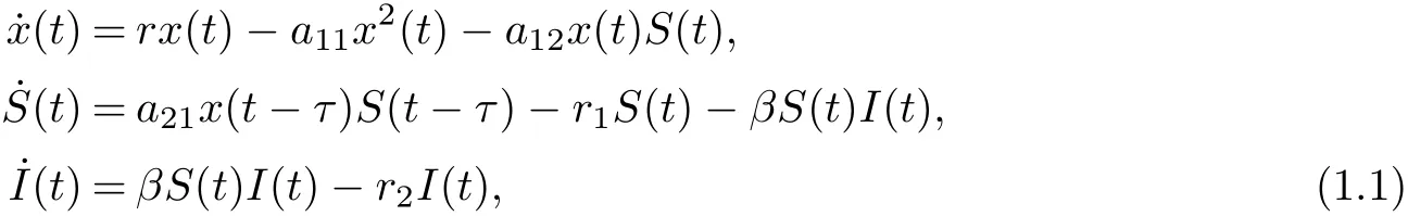
where x(t),S(t),I(t) denote the densities of the prey, the susceptible predator and the infected predator population, respectively.

The functional response is a key element in all predator-prey interactions. The functional response refers to the number of prey eaten per predator per unit time as a function of prey density.System (1.1) assumes that the per capita rate of predation depends on the prey numbers only.But there is growing explicit biological and physiological evidence that in some situations,especially when predators have to research for food(and therefore have to share or compete for food),a more realistic model should be based on a functional response which is predator-dependent.Such as , ”ratio-dependent” theory [13-15], and in some cases, the Beddington-DeAngelis type functional response performed even better. The Beddington-DeAngelis functional responsewas introduced by Beddington-DeAngelis et al. [16-17]. It is similar to the well-known Holling type II functional response but has an extra term nS(t)in the denominator which models mutual interference between the susceptible predator. When m > 0, n = 0, the Beddington-DeAngelis functional response is simplified to Holing type II functional response.And when m=0, n>0, it expresses a saturation response.

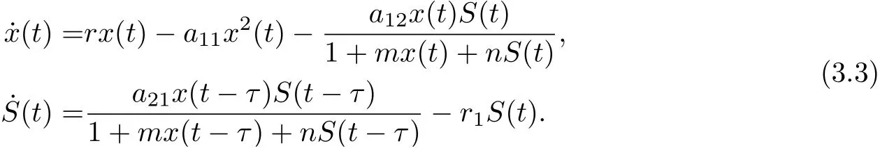
Motivated by the works of Zhang et al. [8]and Beddington-DeAngelis et al. [16-17], in this paper, we are concerned with the combined effects of the disease transmission, Beddington-DeAngelis functional response and time delay due to the gestation of predator on the global dynamics of a predator-prey system. To this end, we consider the following eco-epidemiological model with delay:

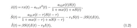
where x(t), S(t) and I(t) denote the densities of the prey, the susceptible predator and the infected predator population, respectively. r is the intrinsic growth rate of prey population without disease, r/a11is the environmental carrying capacity, a12is the capturing rate of the susceptible predators, a21/a12is the conversion rate of nutrients into the reproduction of the susceptible predators by consuming prey, β is the disease transmission coefficient, r1is the natural death rate of the susceptible predators, r2is the natural and disease-related mortality rate of the infected predator. Here, r1≤r2. τ is a time delay representing a duration of τ time units elapses when an individual prey is killed and the moment when the corresponding addition is made to the predator population. All the parameters are positive.

We denote by C the Banach space of continuous functions φ:[?τ,0]→R3with norm

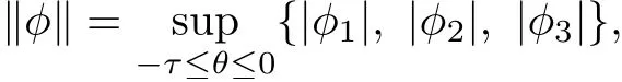
where φ=(φ1, φ2, φ3)∈C. Further, let

The initial conditions for system (1.3) take the form

where φ=(φ1, φ2, φ3)∈C+.

The organization of this paper is as follows. In sec. 2,we present some preliminaries,such as the positivity, and the equilibria of system (1.2). In sec. 3, we consider about the permanence of system (1.2) by using the persistence theory on infinite dimensional systems developed by Hale and Waltman [18]. In sec. 4, by means of suitable Lyapunov functionals and Lasalle’s invariance principle, we establish sufficient conditions for the global asymptotic stability of the interior equilibrium and the disease-free equilibrium of system (1.2). Finally, the paper ends with a summary and discussion.

§2. Preliminaries

In this section, we show the positivity of solutions and the equilibria of system (1.2).

2.1 Positivity of solutions

Theorem 2.1Suppose that (x(t),S(t),I(t)) is a solution of system (1.2) with initial conditions (1.3). Then x(t)>0, S(t)>0 and I(t)>0 for all t ≥0.

ProofFrom the first and last equation of system (1.2), we have

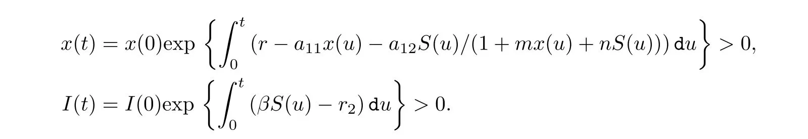
Hence, x(t) and I(t) are positive.

To show that S(t)is positive on[0,∞),suppose that there exists t2>0 such that S(t2)=0,and S(t)>0 for t ∈[0,t2). Then ˙S(t2)≤0. From the second equation of (1.2), we have

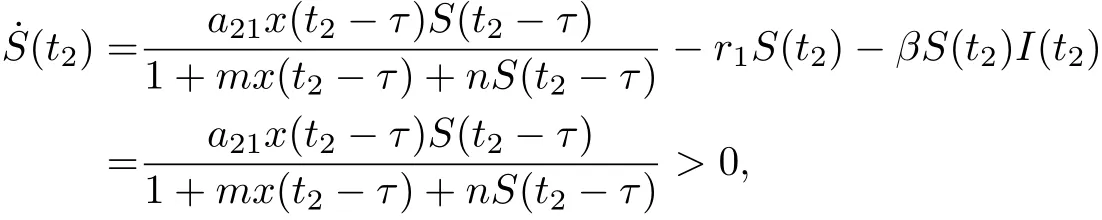
which is a contradiction.

Next, we will give the equilibria of system (1.2).

2.2 equilibriaEquilibria of system (1.2) are obtained by setting the right side of three equations of (1.2) to zeros. Doing this, we get four equilibria in general.

(i) The trivial equilibrium E0=(0,0,0).

(ii) The predator-extinction equilibrium E1=(r/a11,0,0).

(iii) The disease-free equilibrium E2=(x2,S2,0), where

Obviously, if

(H1) a21?mr1>a11r1/r,

then x2>0, S2>0.

(iv) The interior equilibrium E?=(x?,S?,I?), where

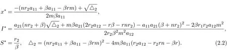
It can be seen that if

then system (1.2) has a interior equilibrium E?.

§3. Permanence

In this section, we consider about the permanence of system (1.2).

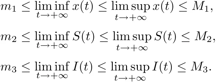
Definition 3.1System (1.2) is said to be permanent (uniformly persistent) if there are positive miand Mi(i=1,2,3)such that each positive solution(x(t),S(t),I(t))of system(1.2)satisfies

Let X be a complete metric space with metric d. Suppose that T is a continuous semiflow on X, that is, a continuous mapping T :[0,+∞)×X →X with the following properties

where Ttdenotes the mapping from X to X given by Tt(x)=T(t,x).

The distance d(x,Y) of a point x ∈X from a subset Y of X is defined by d(x,Y)=infy∈Yd(x,y).

Recall that the positive orbit γ+(x) through x is defined asand its ω?limit set is ω(x)=Define Ws(A)the strong stable set of a compact invariant set A as

Suppose that X0is open and dense in X and X0∪X0= X, X0?. Moreover, the C0-semigroup T(t) on X satisfies

Let Tb(t)=T(t)|X0and Abbe the global attractor for Tb(t).

Lemma 3.1rm(Hale and Waltman[19])Suppose that T(t)satisfies(3.1). If the following hold

(i) there is a t0≥0 such that T(t) is compact for t>t0;

(ii) T(t) is point dissipative in X; and

Then X0is a uniform repeller with respect to X0, that is, there is an ε > 0 such that for any x ∈X0,

In order to study the permanence of system (1.2), we also need following result.

Lemma 3.2There are positive constants M1and M2such that for any positive solution(x(t), S(t), I(t)) of system (1.2) with initial conditions (1.3),

ProofLet(x(t),S(t),I(t))be any positive solution of system(1.2)with initial conditions(1.3). Set

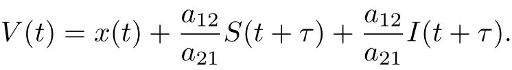
Calculating the derivative of V(t) along positive solution of system (1.2), we get

where M1=which yields≤M1. If we choose M2= a21M1/a12, then(3.2) follows. This complete the proof.

We are now in a position to state and prove our result on the permanence of system (1.2).

Theorem 3.1If βS2>r2and (H1) hold, then system (1.2) is permanent.

ProofLet C+([?τ,0],R3+)denote the space of continuous functions mapping[?τ,0]into R3+. Define

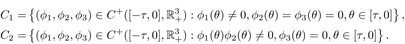
Denote C0=C1∪C2, X =C+([?τ,0],R3+) and C0=intC+([?τ,0],R3+).

In the following, we verify the conditions in Lemma 3.1 are satisfied. By the definition of C0and C0, it is easy to see that C0and C0are positively invariant and the conditions (i) and(ii) in Lemma 3.1 are clearly satisfied. Thus, we need only to show that the conditions (iii)and (iv) hold. Clearly, system (1.2) possesses two constant solutions in C0:corresponding, respectively, to x(t) = r/a11, S(t) = 0, I(t) = 0 and x(t) = x2, S(t) = S2,I(t)=0.

We now verify the condition (iii) of Lemma 3.1. If (x(t),S(t),I(t)) is a solution of system(1.2) initiating from C1, then ˙x(t)=rx(t)?a11x2(t), which yields x(t)→r/a11as t →+∞. If(x(t),S(t),I(t)) is a solution of system (1.2) initiating from C2with φ1(θ) > 0 and φ2(θ) > 0,then we have

Using Lemma 3.1 and Lemma 3.2, it is not difficult to prove that if (H1) holds, then system(3.3) is uniformly persistent. Noting that C1∩C2=?, it follows that the invariant setsandare isolated. Hence,is isolated and is an acyclic covering satisfying the condition(iii) in Lemma 3.1.

§4. Global Stability

In this section, we give some sufficient conditions for global stability of the interior equilibrium E?and the disease-free equilibrium E2, respectively. The method of proofs is to use global Lyapunov functional and Lasalle’s invariance principle.

Theorem 4.1If the interior equilibrium E?of system (1.2) exists, then E?is globally asymptotically stable provided that

ProofAssume that (x(t),S(t),I(t)) is any positive solution of system (1.2) with initial conditions (1.3). Denote φ(x(t),S(t))=Define

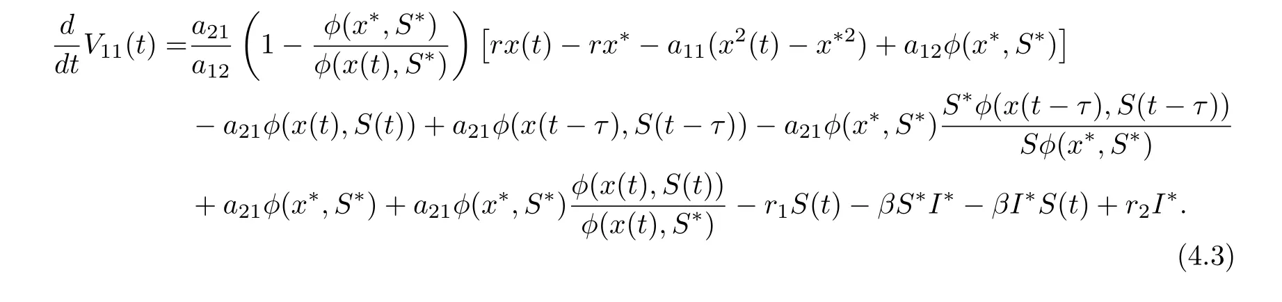
Calculating the derivative of V11(t) along positive solutions of system (1.2), it follows that

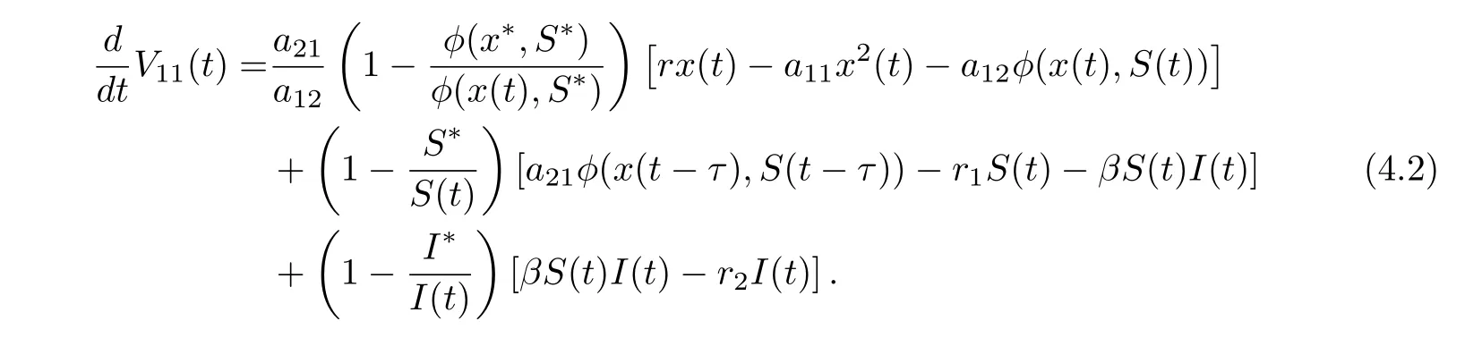
On substituting rx??a11x?2?a12φ(x?,S?) = 0, a21φ(x?,S?)?r1S??βS?I?= 0 and βS?=r2into Eq. (4.2), we derive that

Define

Then

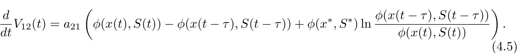
Set V1(t)=V11(t)+V12(t). It follows from (4.1) (4.4) and (4.5) that

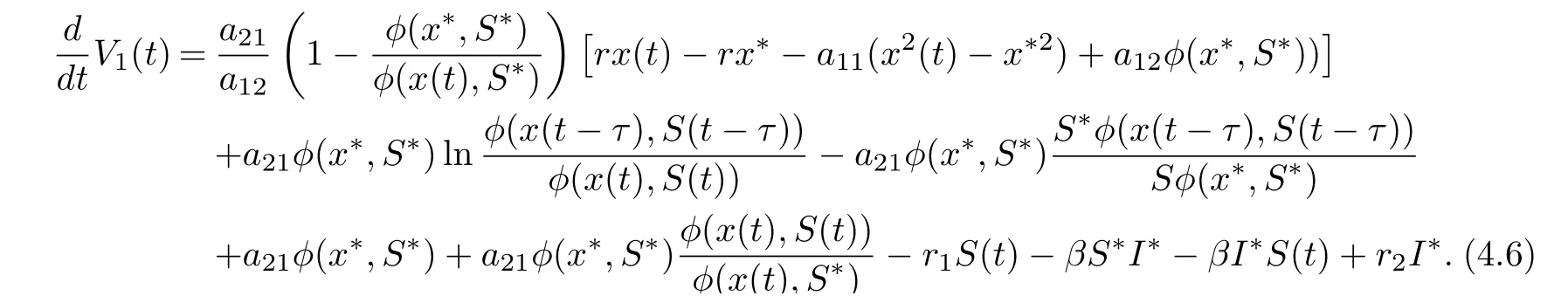
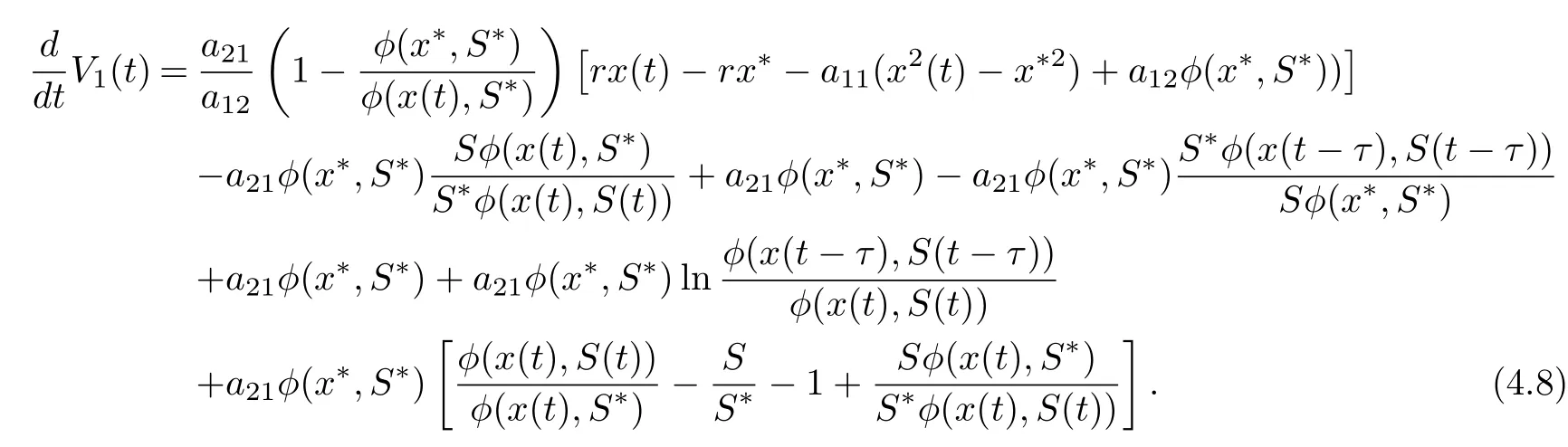
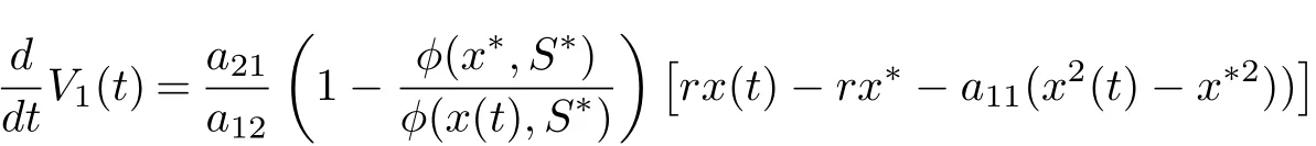
Collecting terms of Eq. (4.6), we get

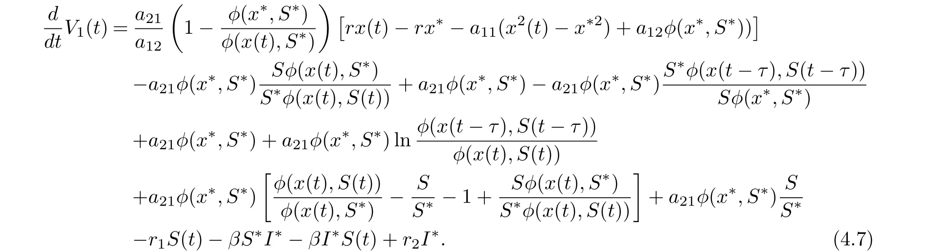
On substituting a21φ(x?,S?)=r1S?+βS?I?and βS?I?=r2I?into Eq. (4.7), we derive that

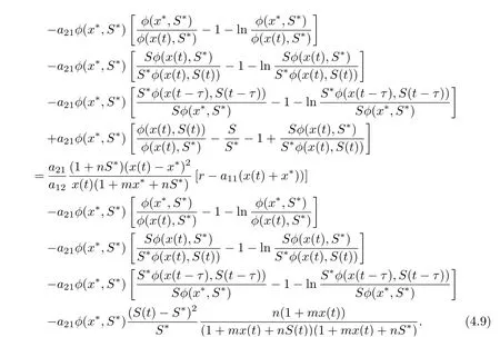
Noting that

we derive from (4.8) that

Because (H2) holds, there is a constant T >0 such that if t ≥T, x(t)>r/(2a11). In this case,we have that, for t ≥T,

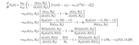
with equality if and only if x = x?. Note that the function f(x) = x ?1 ?ln x is always non-negative for any x>0, and f(x)=0 if and only if x=1. Therefor, we have that if t ≥T,˙V1(t) ≤0, which equality if and only if x = x?,S = S?. We now look for the invariant subset M within the set

Since x = x?,S = S?on M, we obtain from the second equation of system (1.2) that 0 =which yields I =I?. Hence, the only invariant set in M = {(x,S,I) := 0} is M = (x?,S?,I?). Therefore, the global asymptotic stability of E?follows from Lasalle’s invariance principle for delay differential systems[18]. This completes the proof.

Theorem 4.2If βS2?r2<0 and (H2) hold, the disease-free equilibrium E2(x2,S2,0) is globally asymptotically stable.

ProofAssume that (x(t),S(t),I(t)) is any positive solution of system (1.2) with initial conditions (1.3). Denote

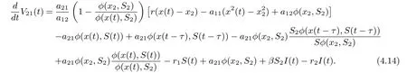
Calculating the derivative of V21(t) along positive solutions of system (1.2), it follows that

On substituting rx2?a11?a12φ(x2,S2)=0 and a21φ(x2,S2)=r1S2into Eq. (4.13), we derive that

Define

Then

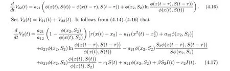
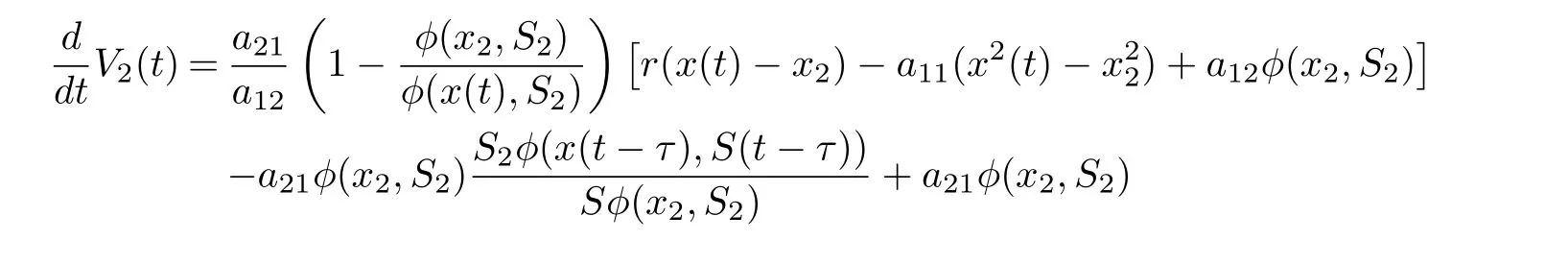
Collecting terms of Eq. (4.17), we get

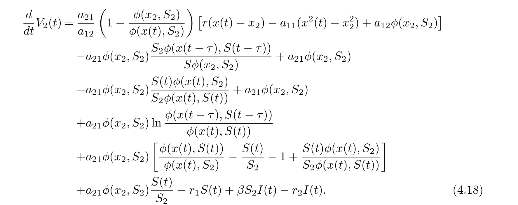
On substituting a21φ(x2,S2)=r1S2into Eq. (4.18), we derive that

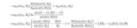
Noting that

we derive from (4.19) that

Hence, if follow from (4.21) that if βS2?r2< 0 and (H2) hold, then≤0 for t ≥T,with equality if and only if x = x2,S = S2,I = 0. It shows that the only invariant set in M = {(x,S,I) := 0} is M = {(x2,S2,0)}. Using Lasalle’s invariance principle for delay differential systems [18]. This completes the proof.

§5. Discussion

In this paper, we have investigated the global dynamics of a delayed predator-prey model with a transmissible disease spreading among the predator population. We noted that system(1.2) has no intra-specific competition terms in the second and the third equations. In this situation, under what conditions will the global stability of a feasible equilibrium of system(1.3) persists independent of the time delay due to the gestation of the predator? To solve this problem, by using Lyapunov functionals and Laselle’s invariance principle, we established global asymptotic stability of the interior equilibrium and the disease-free equilibrium of the system,respectively. According to Theorem 4.1,we can see that if the prey population is always abundant enough, the interior equilibrium of system (1.2) is globally asymptotically stable. By Theorem 4.2, we see that if the susceptible predator population S2< r2/β, that means, the susceptible predator population is not too large, then the disease-free equilibrium of system(1.2) is globally asymptotically stable. In this case, the infected predator will become extinct.