SHI Ren-kun

(Department of Mathematics, College of Science, Hohai University, Nanjing, 210098, China)

Abstract:In this paper, the Cauchy problem of the classical Keller-Segel chemotaxis model with initial data of large mass is considered. By the Green’s function method and scaling technique, we prove that ifand less than some constant, then the problem always admits a unique global classical solution, even when the initial mass is large. Moreover, the decay rates of the classical solution are also obtained.

Key words: Chemotaxis; Keller-Segel; Large mass; Global existence; Decay rate

§1. Introduction

In this paper, we consider the following Cauchy problem of the Keller-Segel model:

where u(x,t) and v(x,t) denote the concentrations of the cells and the chemoattractant, respectively; γ > 0 is a constant and χ > 0 represents the chemoattractant sensitivity; κ = 0 or 1.

The Keller-Segel model is the most famous chemotaxis model proposed by Keller and Segel[1]in 1970s, which is used to describe the movements of cells, bacteria or organisms in response to some chemical signals. One prominent feature of the model is the competition between diffusion and cross-diffusion, which leads to various interesting issues of mathematics such as blow-up, boundedness, global existence, and critical mass phenomenon. In summary, the classical solution of the model exists globally and is uniformly bounded when n=1 (see [2-3]),whereas when n ≥3, the finite time or infinite time blow-up may occur even for small initial data (see [4-6]). The case of n=2 is more interesting due to the critical mass phenomenon. It is proved in[5,7]that the solution of(1.1)exists globally when m:=that blows up in finite time. Similar results hold true for the homogeneous Neumann initial-boundary value problem but with a different mass threshold(see in[8-13]). For more literature about the model,one can refer to the references cited therein and the review articles [14-17].

The results above are classical, from which we can see that the mass m plays an important role in studying large time behavior of the solution, especially when n=2. Roughly speaking,for large initial mass, the diffusion is not strong enough to prevent the aggregation of cells.However,whether all initial data with large mass can lead to the finite time or infinite time blowup in high dimensions,to the best of the author’s knowledge,is still unclear. This motivates me to study the problem(1.1)for large initial mass. It is proved in this paper that ifandare less than some constant which depends only on n,p,χ and γ,then the problem(1.1)always admits a unique global classical solution,even when the initial massis large.Moreover, the decay rates of the classical solution are also obtained. This implies that even for large initial mass, if the initial density of cells is sufficiently small almost everywhere and the initial distribution of the chemoattractant is relatively homogeneous spatially, then the chemotactic collapse cannot happen.

Before showing the result, we first give some notations in the paper.

NotationsThroughout the paper, we denote generic constants by C which may vary line by line according to the context.represents the usual Sobolev space, and the Lpnorm of a function is denoted byfor convenience. G(x,t) =is the heat kernel.

The main result is stated as follows.

Theorem 1.1Let n ≥2. Suppose that the initial data (u0,κv0) is nonnegative andfor some p ∈(n,∞). Then there exits a constant c depending only on n and p, such that if

and

then the Cauchy problem (1.1) admits a unique global classical solution (u,v) ∈C∞(Rn×(0,∞)), and for all 1 ≤q ≤∞, it satisfies

Remark 1.2 When κ = 0, the condition (1.2) always holds true, and thus only the condition (1.3) is needed.

The rest of the paper is arranged as follows. In Section 2, We show the local existence and regularity of the solution, and establish some a priori estimates. In Section 3, we give the proof of Theorem 1.1.

§2. Local Existence and Some A Priori Estimates

In[18],the authors proved the local existence and regularity of the solution to an attractionrepulsion chemotaxis system. In fact, we can follow the ideas therein exactly to prove the following result.

For simplicity, we omit the proof of Lemma 2.1 here.

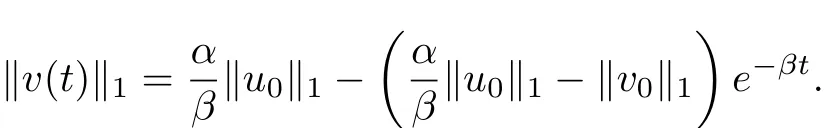
Lemma 2.2 Suppose that (u,v) is a solution of (1.1) which exists in [0,Tmax) with Tmax∈(0,∞]. Then it holds

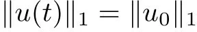
and

From this lemma, we only need to prove the boundedness ofin order to obtain the global existence. Actually, we can prove the following results.

Lemma 2.3 Suppose that (u,v) is the solution of (1.1) with κ = 1 and the initial datafor p ∈(n,∞). Let

Then if it holds that

Proof Now let

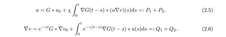
We first make some estimates for Q1and Q2, which are needed for the estimates of u. For the term Q1, it holds that

For Q2, it f ollows from (2.4) that

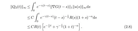
and meanwhile it holds

(2.9) and (2.10) yield that

where

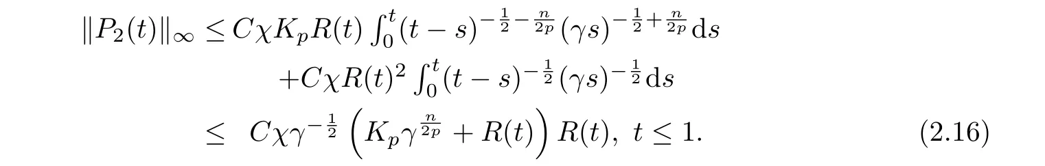
Now we proceed to estimate P2. Here, two different cases, t ≤1 and t > 1, are considered,respectively. Firstly, let us consider the case of t ≤1. By Young’s inequality, we can obtain from (2.7) and (2.8) that

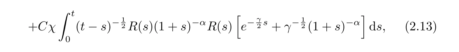
where p?satisfies=1. Then by using the inequalities that

and

we canderive from (2.13) that

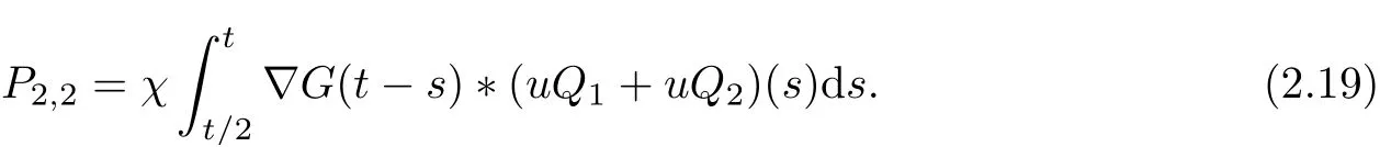
Next we consider the case of t>1. We divide P2into two parts:

where

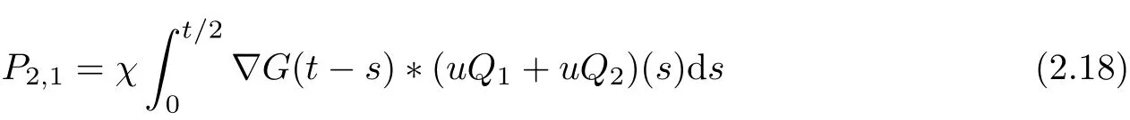
and

For P2,1, it follows from Young’s inequality that

From (2.7), we can derive that

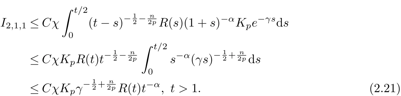
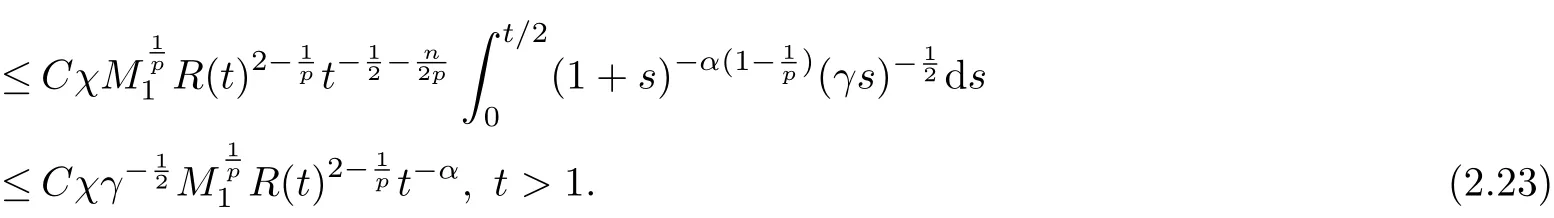
Here,we also used the fundamental inequality(2.14). Next by using(2.8)and the interpolation inequality

we can get from (2.20) that

The collection of (2.20), (2.21) and (2.23) gives that

Now to estimate P2,2from (2.19). By using Young’s inequality, and from (2.7) and (2.8), we have

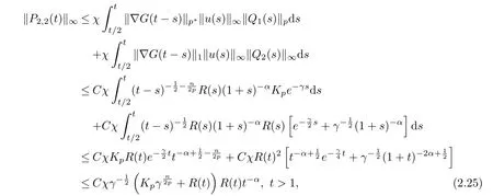
where in deriving the last inequality we used (2.14) and (2.15) again. Then it follows from(2.16), (2.24) and (2.25) that

for all t ≥0. Finally, we collect (2.5), (2.11), (2.26) and (2.4) to get that

By continuity of R(t), it is easy to see from (2.27) that if

then it holds for all t ≥0 that

Hereto the proof is completed.

Lemma 2.3 asserts that for the parabolic-parabolic case,has an upper bound under the assumption (2.2). For the parabolic-elliptic case, it holds a similar result.

Lemma 2.4[κ=0]Suppose that (u,v) is the solution of (1.1) with κ=0 and the initial data u0∈L1(Rn)∩L∞(Rn). Let

Then if it holds that

ProofThe proof is similar to that of LEMMA 2.3. We only need to change the estimates of ?v by

where C depends only on n,and Kγ(x)=G(x,s)ds is the kernel of the Bessel potentialsee in E.M. Stein [19, Ch. V, Sec 3.1].

§3. Proof of the Main Theorem

In this section, we prove Theorem 1.1 based on Lemma 2.3 and Lemma 2.4.

Now we introduce new scaling transforms by

It iseasy to derive that (uλ,wλ) satisfies

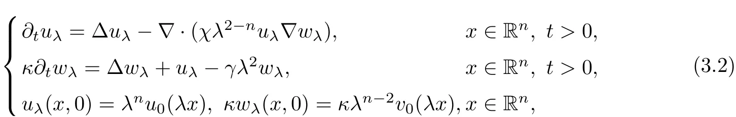
if (u,v) is the solution of (1.1). Obviously, the problem (1.1) is globally solvable if and only if(3.2) is globally solvable for some fixed positive number λ.

Proof of Theorem 1.1We first consider the case of κ = 1. Applying Lemma 2.3 to the system (3.2) and from Lemma 2.1, we know that the transformed problem (3.2) is globally solvable and it satisfies

if the following holds:

where

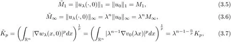
and

Inserting (3.5)-(3.8) into (3.4) and letting λnM∞=M1, we get

Therefore, if it holds that

and

then (3.9) holds true, which means that the problem (3.2) with λ =is globally solvable and admits the decay estimate(3.3). Hereto we have proved that there exists a constant c depending only on n and p, such that the problem (1.1) with κ=1 admits a global classical solution under the conditions (1.2) and (1.3). And furthermore, it holds for all t ≥0 that

The decay rate in(3.12)is not optimal,but it is sufficient for us to derive the optimal L∞decay rate and then to verify (1.4). By Young’s inequality, (2.5) and (2.6) lead to

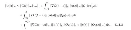
Using (2.7), (2.8) and (3.12), it follows from (3.13) that

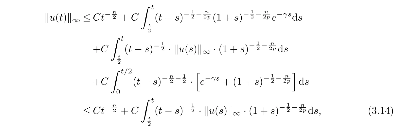
where we have used the boundedness ofandNow using (3.12) again, we can get from (3.14) that

This estimate, together with the boundedness of, yields that

Otherwise, using (3.16) in (3.14) leads to

After repeating the procedure at most[p]times,we can derive(3.17). Then from the Duhamel’s principle

we have

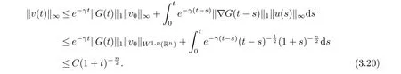
Then (1.4) just follows from the interpolation inequality

Now we only need to prove the theorem for κ = 0. In fact, we can follow the procedure above exactly to give the corresponding proof by applying Lemma 2.4 instead. For simplicity,it is omitted here. The proof is completed.