Keywords:tunneling time,B¨uttiker–Landauer time,Bohm ian time

1.Introduction

The tunneling time problem is almost as old as quantum mechanics itself[1]and has been a subject of intense theoretical debate for many years.[2–15]Recently,progress in attosecond science has allowed for a measurement of tunneling time in the so-called attoclock experiments.[16–26]However,there are considerable controversies in the interpretation of the attoclock experiments.Some investigations have supported a nonzero tunneling delay time,[17,19,26]while others supported a zero tunneling delay time.[27–30]

On the theoretical side,there is still no consensus on the def inition of tunneling time.The Larmor clock was proposed by Baz’[3]and Rybachenko[4]to measure tunneling time.This idea is to use spin polarized electrons and a potential barrier w ith a constant magnetic f ield inside,considering the rotation of the spin in the plane that is perpendicular to the magnetic f ield can def ine a time.B¨uttiker[6]recognized that the Larmor time is equal to the dwell time calculated by the ratio of integrated probability density over the barrier region to the incident f lux.The identity relation between Larmor timeand dwell time isalso fulf illed for apotential barrier of arbitrary shape[11]and in the relativistic case.[10]B¨uttiker also pointed out that the main effect of the magnetic f ield in lamor precession is to align the spin w ith the f ield.Thus,the barrier preferentially transm its a particle w ith spin parallel to the magnetic f ield,which can be described by the B¨uttiker–Landauer time.[6]The B¨uttiker–Landauer time τBL[5]describes the time spent by the particle to travel from the entrance point x1to the exit point x2under the barrier V(x).Within the Wentzel–Kramers–Brillouin(WKB)approximation,the general def inition of B¨uttiker–Landauer time is,[5]where p(x)=is the momentum of particlew ith thekinetic energy E under thebarrier.A fterwards,Sokolovski and Baskin constructed a single complex time by Feynman path-integral technique,which can elegantly combine the Larmor timeand the B¨uttiker–Landauer time.[31]Very recently,we proposed a def inition of quantum travel time which provides a reasonable interpretation of the tunneling delay time measured by attoclock experiment and bridges thegap between itand the B¨uttiker–Landauer time.[32]This quantum travel time can also provide a reasonable description in the case of very thin barrier where the B¨uttiker–Landauer time isnot well def ined.

A lthough there are many conf licting def initions of tunneling time in conventional quantum mechanics,Bohmian mechanics[33,34]privileges the time that the Bohm ian trajectory spends between theentranceand exit points of the potential barrier.[35]Recently,it has been found that the Bohmian timedoesnotcorrespond to the tunneling time,butagreesw ith the resonance lifetime of a bound state.[35]

In thispaper,we further explore the relationship between the new ly introduced quantum travel time w ith other def initionsof tunneling time(Larmor time,B¨uttiker–Landauer time,and Bohmian time)in one-dimension rectangular tunneling process.In Section 2,we give a brief calculation about the one-dimension rectangular barrier tunneling and show the dif-ferent def initions of tunneling time(quantum travel timeτt,tRe,tIm;the Larmor time tLMand associated times(tx,ty,and tz)).In Section 3,we investigate the relationship between different tunneling times and f ind that the real quantum travel time tReis equal to the Bohm ian time tBohmian,and the total quantum travel timeτtcan bridge the connection between the time txand the B¨uttiker–Landauer timeτBL.

2.Theoreticaldef inition of tunneling time

2.1.Rectangular barrier tunneling

Consider a particle with kinetic energy E=ˉh2k2/2m moving along the x-axisand interactingwith a rectangularbarrier of height V0and w idth d centered at x=0,as shown in Fig.1.Thewave function of the particlewithin different regions(I,II,and III)can bew ritten as

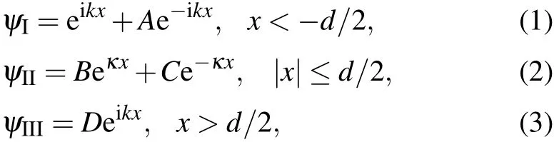
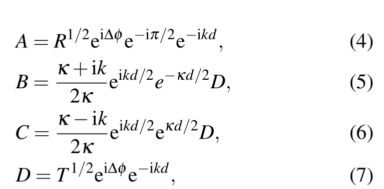
where T is the transmission probability

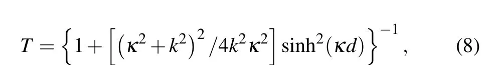
andΔθis thephase changed across thebarrierwith

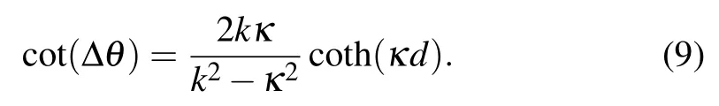
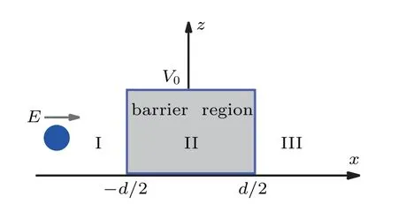
Fig.1.Schematic diagram:a particle with kinetic energy E moves along the x-axis and interactswith a rectangular barrierwith height V0 and w idth d centered at x=0.

2.2.Quantum travel time

In quantum mechanics,themomentum operator iswell def ined,thus thequantum travel time isintroduced by analogy with the classical travel time[32]

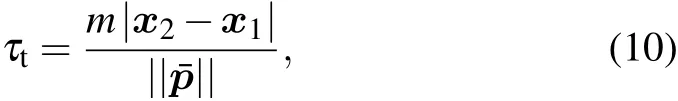
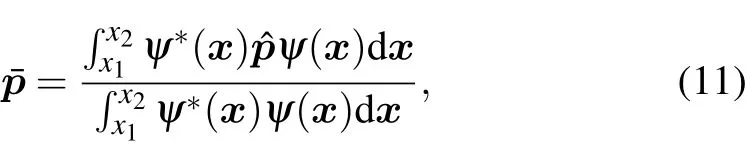
where m is themass of the particle and||···||meansmaking themodulaof“···”.Theaveragemomentumˉp of the particle during itsstaywithin thebarrier region(x1,x2)canbeobtained by calculating the expected value of themomentum operator ?p=-iˉh?where

The averagemomentum divided by themass of particle gives the average velocity of the particle within the barrier region.We def ine theaverage velocity as follows:

According to thedef inition ofquantum travel time in Eq.(10),we can also def ineanother two different times

We can easily obtain the relationship between the three times,tRe,tIm,andτt,from Eq.(16)whereψ(x)is thewave function of the particlewithin the region(x1,x2).

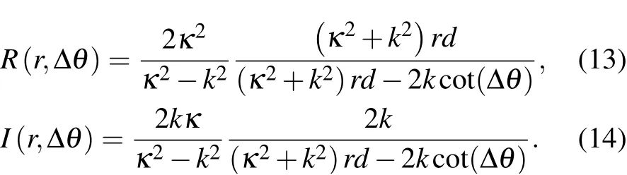
By combining Eqs.(5)–(9)and substituting Eq.(2)into Eq.(11),we can obtain theaveragemomentum of the particle within thebarrier region[32]

2.3.Larmor timeand associated times

Considering an incident particle with x-direction polarized spin tunneling through a barrier region within a constant z-directionmagnetic f ield B,theparticlew illexperiencea Larmorprecession.[6]For the transm ittedwavefunctionof theparticle,we can calculate the expectation valuesof spin in three different directions:＜Sx＞,＜Sy＞,and＜Sz＞.The Larmor time tLMis the average time spentby the particle inside the barrier,which is given by the degree of precession in the y-direction Sy[10,14]

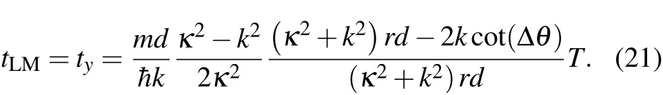
whereωL=B/2 is the Larmor frequency(the atom ic units(a.u.)are used). By combining the def initions of r and cot(Δθ),we canw rite the Larmor time tLMas follows:

Since the particle tunneling through the barrier can also acquire a spin componentparallel to themagnetic f ield,[6]the z-direction precession of spin＜Sz＞can also def ine a time tz[6,14]

This time tzcan be rew ritten as For the expectation value of spin in the x-direction＜Sx＞,a time txis also def ined,[6]which satisf ies the relationship as follows:

3.Relationship between different tunneling times

3.1.Thequantum travel tim es t Re,t Im,andτt

First,we discuss the behavior of the quantum travel time in two opposite lim iting cases.In the lim it of the very thin barrierκd?1,the coeff icients on the right side of Eq.(12)can be approximated to R(r,Δθ)≈1 and I(r,Δθ)≈0.In the opposite lim itofopaquebarrierκd?1,wehave R(r,Δθ)≈0 and I(r,Δθ)≈1.Accordingly,we can obtain

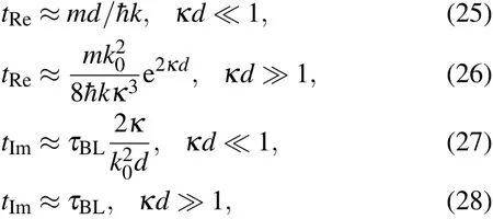
whereτBL=md/ˉhκis the B¨uttiker–Landauer time.Thus,for the very thin barrierκd?1,the timeτtismainly determ ined by the time tRe,i.e.,τt≈tRe≈md/ˉhk,which means that a classical particle passes through a distance d withmomentumˉhk.While in the case of opaque barrierκd?1,tt≈tImapproaches the B¨uttiker–Landauer time md/ˉhκwhich isalso obtained in the lim itof opaquebarrier.[5]Thesebehaviorsof the threequantum travel times can be clearly seen in Fig.2.

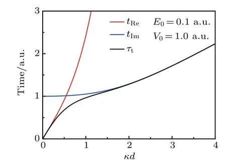
Fig.2.A comparison between time t Re,t Im,andτt as a function of κd with E=0.1 a.u.and V0=1.0 a.u.The atom ic unitsare used withe=m=ˉh=1.

3.2.The Bohm ian tim e t Bohm ian,the Lam or time t LM,and time t Re

The Bohmian time is def ined as the time required for a Bohm ian trajectory to pass the region between the two classical turning points x1and x2[34,35]

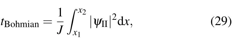
where J=ˉhkT/m is thestationary probability f lux.Aftersubstituting Eq.(2)into Eq.(29),we obtain

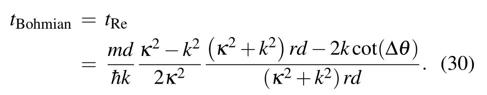
The Bohmian timewas found to be related to the resonance lifetimeofabound state,[35]which can be calculated from the resonancew idthsΓtaken from Ref.[36].Comparing Eq.(21)with Eq.(30),we can obtain tBohmian=tRe=tLM/T=ty/T.Thus,the time tReisalso related to the decay ratesof quasistationary statesand ref lects the resonance lifetime.

3.3.The B¨uttiker–Landauer timeτBL,the tim es tx,andτt

The B¨uttiker–Landauer timeτBLisbased on the onsetof the“cross-over”regime between pure tunneling and tunneling while absorbing one ormore photons from the oscillating f ield.[5]B¨uttiker and Landauer argued that this timeτBLcan determine the actual barrier transversal time.In Section 3.1,we show that the timeτtismainly determ ined by the time tImfor an opaque barrier,which isequal to the B¨uttiker–Landauer timeτBL.In Fig.3,we show the comparison betweenτBL=md/ˉhκand tImfor different kinetic energies E

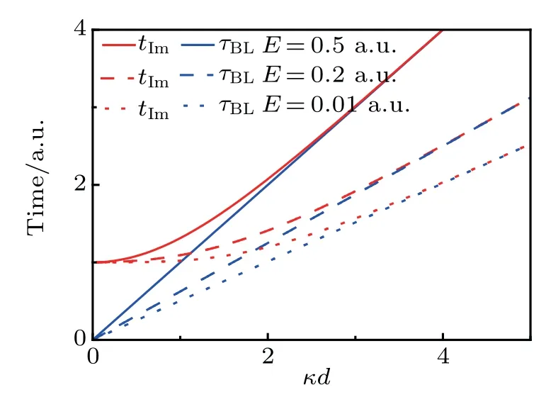
Fig.3.A comparison between time t Im and the B¨uttiker–Landauer time τBL asa function ofκd with E=0.5 a.u.and V0=1.0 a.u.Theatom ic unitsareusedwith e=m=ˉh=1.

B¨uttiker proposed that the time tx(Eq.(24))can also be used as the barrier traversal time.In Fig.4,we show a comparison between the times tx(red line),τBL(blue line),and τt(black line)under differentkinetic energiesof the particle.Although both the time txand the B¨uttiker–Landauer timeτBLcan be treated as barrier traversal time,there is a difference between them,especially when the dimensionless parameter κd is not very large.The difference increases as the kinetic energy of the particle decreases.Itis interesting that thequantum travel timeτtcan perfectly retrieve txandτBLin two opposite lim its,regardlessof the particle energy.As seen in Fig.4,τtis equal to the time txwhenκd is small.Andτthas an asymptotic behavior sim ilar to the time tx,i.e.,approaching the f inite value 1/V0in the lim it that the kinetic energy of the particle and thew idth of the potential barrier tends to zero at the same time.In the opposite limit,τtperfectly coincides with the B¨uttiker–Landauer timeτBLwhenκd＞3.While in the range1＜κd＜3,thevalueof timeτtjust fallsbetween the two times:txandτBL.Thequantum travel timeτtiscomposed of two parts:time tReand time tIm.The time tImcharacterizes the quantum property of the tunneling process.The time tReref lects the timeneeded by theentirewavefunction of the particle to tunnel through thebarrier,which includes the inf luence of the transmission probability.In the condition that thew idth of barrier approaches zero,the transm ission probability tends to one.Thus,the time tRetends to the classical time,which means the time thata classicalparticleneeds to pass through a distance d.The time txisalso composed of two parts:tyand tz.The time tyis related to the time tRe(tRe=ty/T).The time tzis derived under inf initesimal f ield,which can be approximated toτBLunderopaquebarrierapproximation.While in our def inition of quantum travel time,the time tImisequivalent to the B¨uttiker–Landauer timeτBLunder opaque barrierapproximation.Thus,we bridge the connection between the time txand the B¨uttiker–Landauer timeτBLthrough the quantum travel timeτt.

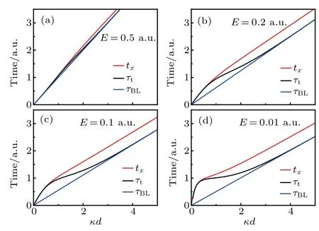
Fig.4.The time tx,the timeτt,and the B¨uttiker–Landauer timeτBL as a function ofκd with(a)E=0.5 a.u.,(b)E=0.2 a.u.,(c)E=0.1 a.u.,and(d)E=0.01 a.u.The heightof the potentialbarrier V0=1.0 a.u.is the same in(a),(b),(c),and(d).The atom ic units are used withe=m=ˉh=1.

4.Conclusion

In conclusion,based on a new def inition of quantum travel time,we bridge the connections between different tunneling times(τBL,tBohmian,and tx)in theone-dimensional rectangularbarrier tunneling.The time tReisequal to theBohmian time tBohmian,which is related to the resonance lifetime of a bound state.The timeτtisa generalized traversal timewhich cannot only retrieve the B¨uttiker–Landauer time forκd＞3 butalso equal the time txwhenκd issmall.In the casewhere the kinetic energy of the particle and thew idth of the barrier tend to zero at the same time,then time txand timeτthave the same limiting value1/V0.

Referencesof the particle.It can be seen that the time tImperfectly coincideswith the B¨uttiker–Landauer timeτBLin the condition of κd＞3.However,there is obvious difference between them in the regionκd＜3.The time tIm,in the limit of thin barrier,i.e.,d→0,approaches a f inite value 1/V0regardless of the kinetic energy of the particle.This can beunderstood from the uncertainty relation of the time and energyΔEΔt～ˉh considering that for a particle to pass through the barrier with a height V0,the time itneeds is about1/V0.It is noted that the B¨uttiker–Landauer timeτBLis obtained in the opaque barrier approximation,[5]while in the lim itof very thin barrier,there isnowell-def ined B¨uttiker–Landauer time.

[1]Maccoll L A 1932 Phys.Rev.40 621[2]Smith FT 1960 Phys.Rev.118 349

[3]Baz’A I1967 Sov.J.Nucl.Phys.4 182

[4]Rybachenko V F 1967Sov.J.Nucl.Phys.5 635

[5]B¨uttikerM and Landauer R 1982 Phys.Rev.Lett.49 1739

[6]B¨uttikerM 1983Phys.Rev.B 27 6178

[7]Landauer R 1989Nature 341 567

[8]Hauge EH and St?vneng JA 1989Rev.Mod.Phys.61 917

[9]Landauer R and Martin T 1994Rev.Mod.Phys.66 217

[10]Bracher C 1997 J.Phys.B 30 2717

[11]LiZ J,Liang JQ and Kobe D H 2001 Phys.Rev.A 64 042112

[12]M cdonald C R,Orlando G,Vampa G and Brabec T 2013 Phys.Rev.Lett.111 090405

[13]Orlando G,M cdonald C R,Protik N H and Brabec T 2014 Phys.Rev.A 89 014102

[14]Landsman A Sand KellerU 2015Phys.Rep.547 1

[15]Teeny N,Yakaboylu E,Bauke H and Keitel CH 2016 Phys.Rev.Lett.116 063003

[16]Eckle P,Pfeiffer A N,Cirelli C,Staudte A,D¨orner R,Muller H G,B¨uttikerM and Keller U 2008 Science 322 1525

[17]Eckle P,Smolarski M,Schlup P,Biegert J,Staudte A,Sch¨off ler M,Muller H G,D¨orner R and Keller U 2008Nat.Phys.4 565

[18]PfeifferAN,CirelliC,SmolarskiM,DimitrovskiD,SamhaM A,Madsen L B and Keller U 2012Nat.Phys.8 76

[19]Landsman A S,Weger M,Maurer J,Boge R,Ludw ig A,Heuser S,CirelliC,Gallmann L and Keller U 2014Optica 1 343

[20]Barth Iand Sm irnova O 2011Phys.Rev.A 84 063415

[21]Pfeiffer A N,CirelliC,Landsman A S,SmolarskiM,DimitrovskiD,Madsen L B and Keller U 2012 Phys.Rev.Lett.109 083002

[22]KlaiberM,Yakaboylu E,Bauke H,Hatsagortsyan K Z and KeitelCH 2013 Phys.Rev.Lett.110 153004

[23]LiM,Liu Y,Liu H,Ning Q,Fu L,Liu J,Deng Y,Wu C,Peng L Y and Gong Q 2013 Phys.Rev.Lett.111 023006

[24]Yakaboylu E,K laiberM and Hatsagortsyan K Z 2014 Phys.Rev.A 90 012116

[25]K laiber M,Hatsagortsyan K Z and Keitel C H 2015 Phys.Rev.Lett.114 083001

[26]Camus N,Yakaboylu E,Fechner L,K laiberM,Laux M,M iY H,Hatsagortsyan K Z,Pfeifer T,Keitel C H and Moshammer R 2017 Phys.Rev.Lett119 023201

[27]Torlina L,Morales F,Kaushal J,Ivanov I,Kheifets A,Zielinski A,ScrinziA,Muller H G,Sukiasyan S,Ivanov M and Smirnova O 2015

Nat.Phys.11 503

[28]NiH,Saalmann U and Rost JM 2016 Phys.Rev.Lett.117 023002

[29]Eicke N and Lein M 2018 Phys.Rev.A 97 031402

[30]Bray AW,EckartSand KheifetsA S 2018Phys.Rev.Lett.121 123201

[31]SokolovskiD and Baskin LM 1987 Phys.Rev.A 36 4604

[32]Hao X L,Shu Z,LiW D and Chen J2019 arXiv:1903.06897[atom-ph]

[33]Wiseman HM 2007New J.Phys.9 165

[34]Bohm D 1952 Phys.Rev.85 166

[35]Zimmermann T,M ishra S,Doran BR,Gordon D Fand Landsman A S 2016 Phys.Rev.Lett.116 233603

[36]Damburg R Jand Kolosov V V 1976 J.Phys.B 9 3149