(School of mathematics and statistics, Chuxiong Normal University, Yunnan Chuxiong, 675000, China)

Abstract：In this paper, applying the method of qualitative analysis of differential equations, we classify the parameter space and phase portraits of a Z2-equivariant planar Hamiltonian vector field of degree 7 and get 33 phase portraits.

Key words：Z2 equivariant property; planar Hamiltonian vector field; singular point; phase portrait

In recent decades, thephase portraits of planarZq- equivariant Hamiltonian vector fields of degree 7 have been studied [1～4], but we still have many works to do . In this paper, we classify the phase portraits of following planar Hamiltonian vector fields of degree 7

(1)

and get 33 phase portraits ,wherekis a positive parameter .

1 Discussion on the Singular Points

Leta=k,b=k+0.2,c=k+0.3,l=k,m=k+0.25 andn=k+0.3, then the system has 49 singular points: (0,0), (±a,0),(±b,0),(±c,0),(0,±l),(0,±m(xù)),(0,±n),(±a,±l),(±b,±l),(±c,±l),(±a,±m(xù)),(±b,±m(xù)),(±c,±m(xù)),(±a,±n),(±b,±n)and(±c,±n).

Because the system (1) is ofZ2- equivariant property, we will discuss the singular points in the first and second quadrants.

The Jacobian of this system is

in which

φ1(x)= -(x2-k2)[x2-(k+0.2)2][x2-(k+0.3)2]-2x2[x2-(k+0.2)2][x2-(k+0.3)2]

-2x2(x2-k2)[x2-(k+0.3)2]-2x2(x2-k2)[x2-(k+0.2)2],

φ2(y)= (y2-k2)[y2-(k+0.25)2][y2-(k+0.3)2]

+2y2[y2-(k+0.25)2][y2-(k+0.3)2]

+2y2(y2-k2)[y2-(k+0.3)2]+2y2(y2-k2)[y2-(k+0.25)2].

Investigating the Jacobians of these singular points, we have the following results:

Theorem1 The singular points (0,0), (±b,0),(0,m),(±a,l),(±c,l),(±b,m),(±a,n)and (±c,n) are center, and the others are saddle points.

2 Phase Portraits of the System (1)

The Hamiltonian of the system is

H(x,y)=[3x8-(12k2+4k+0.52)x6+(18k4+12k2+3k2+0.36k+0.0216)x4]/24

-(k6+k5+0.37k4+0.06k3+0.0036k2)x2/2-(12k6+13.2k5+5.43k4+0.99k3+0.0675k2)y2/24

+[(18k4+13.2k3+3.63k2+0.495k+0.03375)y4-(12k2+4.4k+0.61)y6+3y8]/24.

Obviously, the functionH(x,y) satisfies the following equalities

H(x,y)=H(x,0)+H(0,y),

H(±a,0)=k4[3k4+2k3+0.26k2-6(k+0.2)2(k+0.3)2]/24,

H(±b,0)=-[(k+0.2)8-2(k+0.2)6(2k2+0.6k+0.09)+6k2(k+0.2)4(k+0.3)2]/24,

H(±c,0)=-[(k+0.3)8-2(k+0.3)6(2k2+0.4k+0.04)+6k2(k+0.3)4(k+0.2)2]/24,

H(0,l)=k4[3k4+2.2k3+0.305k2-6(k+0.25)2(k+0.3)2]/24,

H(0,m)=-[(k+0.25)8-2(k+0.25)6(2k2+0.6k+0.09)+6k2(k+0.25)4(k+0.3)2]/24,

H(0,n)=-[(k+0.3)8-2(k+0.3)6(2k2+0.5k+0.0625)+6k2(k+0.25)2(k+0.3)4]/24.

Comparing the Hamiltonians of the singular points, we obtain the following outcomes.

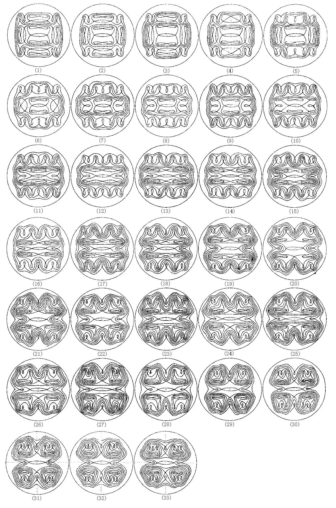
Theorem2 There are 33 phase portraits of system (1) shown in Fig.1 whenkseparately

belongs to the following intervals : (1)k∈(0,0.05), (2)k=0.05, (3)k∈(0.05,0.114716),

(4)k=0.114716, (5)k∈(0.114716,0.17027), (6)k=0.17027,

(7)k∈(0.17027,0.196385), (8)k=0.196385, (9)k∈(0.196385,0.212697),

(10)k=0.212697, (11)k∈(0.212697,0.230318), (12)k=0.230318,

(13)k∈(0.230318,0.242755), (14)k=0.242755, (15)k∈(0.242755,0.269742),

(16)k=0.269742, (17)k∈(0.269742,0.282514), (18)k=0.282514,

(19)k∈(0.282514,0.288958), (20)k=0.288958, (21)k∈(0.288958,0.29392),

(22)k=0.29392, (23)k∈(0.29392,0.304662), (24)k=0.304662,

(25)k∈(0.304662,0.314672), (26)k=0.314672, (27)k∈(0.314672,0.325411),

(28)k=0.325411, (29)k∈(0.325411,0.409808), (30)k=0.409808,

(31)k∈(0.409808,0.484832), (32)k=0.484832, (33)k∈(0.484832,+∞).

Proof We separately use the symbolsh00,ha0,hb0,hc0,h0l,h0m,h0n,hal,ham,han,hbl,hbm,hbn,hcl,hcmandhcmto expressH(0,0),H(±a,0),H(±b,0),H(±c,0),H(0,l),H(0,m),H(0,n),H(±a,l),H(±a,m),H(±a,n),H(±b,l),H(±b,m),H(±b,n),H(±c,l),H(±c,m), andH(±c,n).

Obviouslyhxy=hx0+h0y,h0l0.05,ha0

(1) The Hamiltonians of the singular points satisfy one of the following relations as 0

hcl

hcl

hcl

hcl

and the phase portrait is shown as Fig.1(1).

(2)Ask=0.05, we haveha0=hc0, and the Hamiltonians of the singular points satisfy the relations

hcl=hal

so the phase portrait is shown as Fig.1(2).

(3) The Hamiltonians of the singular points satisfy one of the following relations as 0.05

hal

hal

hal

hal

hal

hal

and the phase portrait is shown as Fig.1(3).

(4)Whenk=0.114716, we getham=h0n, and the Hamiltonians of the singular points satisfy the relations

hal

so the phase portrait is shown as Fig.1(4).

(5) The Hamiltonians of the singular points satisfy one of the following relations as 0.114716

hal

hal

hal

and the phase portrait is shown as Fig.1(5).

(29) The Hamiltonians of the singular points satisfy one of the following relations when 0.325411

hal

hal

hal

hal

so the phase portrait of the system (1) is shown as Fig.1(29).

(30) Whenk=0.409808, the Hamiltonians of the singular points satisfy the relations

hal

and the phase portrait of the system (1) is shown as Fig.1(30).

(31) The Hamiltonians of the singular points satisfy one of the following relationswhen 0.409808

hal

hal

so the phase portrait of the system (1) is shown as Fig.1(31).

(32) Ask=0.484832, the Hamiltonians of the singular points satisfy the relations

hal

so the phase portrait of the system (1) is shown as Fig.1(32).

(33) Ask>0.484832, the Hamiltonians of the singular points satisfy one of the following relations

hal

hal

so the phase portrait of the system (1) is shown as Fig.1(33).

Fig.1(1)～(33) The phase portraits of system (1)