
Seiberg-Witten/Whitham Equations and Instanton Corrections in N=2 Supersymmetric Yang-Mills Theory?
2018-06-11 12:21:14JiaLiangDai戴佳亮andEnGuiFan范恩貴
Jia-Liang Dai(戴佳亮) and En-Gui Fan(范恩貴)
School of Mathematical Science,Fudan University,Shanghai 200433,China
1 Introduction
The solution of exact low energy effective action in N=2 supersymmetric Yang-Mills theory with SU(2)gauge group was obtained by Seiberg and Witten in Ref.[1]and their work have been generalized to the other higher rank gauge group SU(n),SO(n)and Sp(n)without or with matter hypermultiplets in the fundamental representation as well as to the exceptional group.The key analysis in Ref.[1]was that the quantum moduli space of N=2 supersymmetric gauge theories coupled with or without hypermultiplets could be naturally identi fi ed with the moduli space of certain hyperelliptic curves or Riemann surfaces.More specifically,with the help of these hyperelliptic curves we can describe the low energy effective action by a single holomorphic function F called prepotential and the exact solution for the prepotential is completely determined from the period integrals of a meromorphic differential on the hyperelliptic curves.[2?4]In general,the expression of prepotential F in the weakcoupling region may be divided into three parts:classical part Fclass,perturbative part Fpertwhich arises only from one-loop effects,and a sum of n-instanton part Fnin[5?6]
it is well known that various kinds of methods have been developed to derive the prepotential from the Seiberg-Witten curves such as hypergeometric functions,[3]Picard-Fuchs equations[7?12]and the renormalization group type equations,[13]however,their complexity increases rapidly as the rank of the gauge group is large,even without matter hypermultiplets.In addition,another important observation about prepotential was noticed by Nekrasov[14]who introduced a partition function which is the generating function of the integral of equivariant cohomology class on the moduli space of framed instantons and showed[15]that the logarithm of this partition function is the instanton part of the Seiberg-Witten prepotential in N=2 supersymmetric four-dimensional gauge theory with gauge group SU(n).Meanwhile,Nakajima and Yoshioka[16]independently proved Nekrasov’s conjecture using the blowup techniques and Hilbert scheme which relates the Seiberg-Witten curves,prepotential and partition function together.These give a framework for understanding the instantons in gauge theory,integrable systems and representation theory of in finite-dimensional algebras in an intricate way.
On the other hand,it was soon discovered that there exists a deep connection between Seiberg-Witten gauge theory and integrable system.[17?21]Roughly speaking,the Seiberg-Witten solution for the N=2 supersymmetric Yang-Mills theory is equivalent to a homogeneous solution of the Whitham hierarchy as well as the prepotential F corresponds to the logarithm of the Toda’s quasiclassical tau function.In the theory of Whitham hierarchy,there is a new family of variables introduced into the prepotential known as Whitham slow times Tnwhile the Whitham equations parameterized by the slow times characterize the deformations of the Seiberg-Witten curves.Around this time,the RG equations in Seiberg-Witten theory were fi rst derived by Gorsky,Marshakov,Mironov,and Morozov in Ref.[13]with the aid of Whitham hierarchy.Furthermore,based on their work Takasaki pointed out that the deformations by T1are interpreted as the renormalization group flows while the other Whitham deformations may be viewed as generalized RG flows.[22?23]More importantly,it is of great significance to remark that the second derivative of the prepotential F with respect to the slow time Tnleads to the appearance of the Riemann Theta-function.In this sense,after appropriately rescaling the gauge invariant parameters,the T1can be naturally regarded as the dynamical scale Λ which explicitly occurs in the Seiberg-Witten theory and the main RG equations required in this paper are given by[24?25]
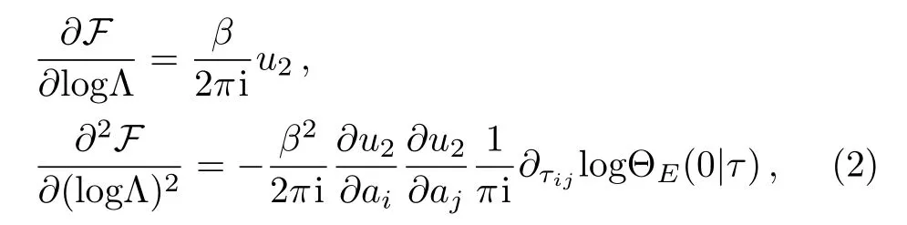
here the symbol ΘE(0|τ)is the Riemann’s theta function associated to the hyperelliptic curve C
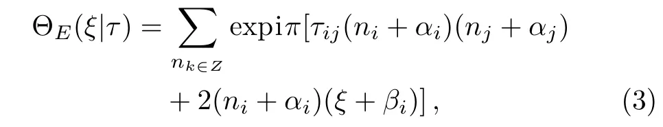
where E=[α;β]Tstands for an even half integer characteristic and in the case of pure SU(n)gauge theory it will be in the form of E=[0,...,0;1/2,...,1/2]T.From the above discussion,there is no difficulty in seeing that one can calculate any desired order instanton correction terms in SU(n)supersymmetric gauge theory by comparing the expansion coefficients of powers of Λ on both sides of Eq.(2)if we insert into the semiclassical expression of the prepotential F.Therefore,one of the most fundamental results of the Seiberg-Witten/Whitham equations is that they provide us a precise description of general recursion relations for any order instanton correction coefficient Fnin terms of the lower order instanton correction terms.It then follows that from this point of view,in principle,we could obtain arbitrary higher order correction coefficient Fnwithout solving the explicit expressions for the Seiberg-Witten periods a,aDwhich is the major feature of this article.
The paper is organized as follows. In Sec.2 we briefly deduce the instanton correction coefficients using the Seiberg-Witten/Whitham equations in the case of SU(2)supersymmetric gauge theory as an illustrative example.In Sec.3 we generalize this approach to the general SU(n)situation and mainly we compute one-and two-instanton correction coefficients in detail,moreover,our results are in agreement with those in Ref.[5].Section 4 contains some conclusions and discussions and Appendix supplies us with relevant calculations and specific proofs we needed in Sec.3.
2 SU(2)Case
Let us first discuss the simplest case of non-abelian SU(2)supersymmetric gauge theory.For the moment due to the instanton effect,it is sufficient to consider the prepotential in SU(2)case without hypermultiplets and the general form of the prepotential F is[3]
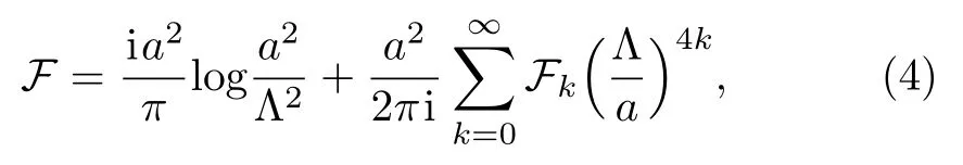
here the first term in Eq.(4)is one-loop expression for the prepotential which does not receive higher order perturbative corrections and the coefficients Fkin second term are constants.Notice that searching for the exact low energy effective action solution is equivalent to evaluating Fkfor all the k,fortunately,the Seiberg-Witten/Whitham equations give us an effective and standard procedure to determine these coefficients.Firstly one has
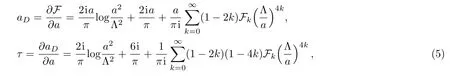
here we set F0=6 which makes the constant coefficient term to be zero and this will be re fl ected in our choice for the normalization of F if we are rescaling Λ appropriately.We apply Eq.(2)to receive

Substituting τ into the Riemann’s theta function(3)we find
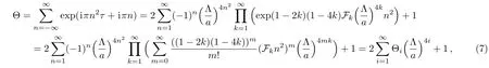
and the derivative of the Riemann’s theta function is

obviously,the Seiberg-Witten/Whitham equations in SU(2)case turns out to be extremely simple

matching the coefficient of(Λ/a)4nterm on both sides of Eq.(9),we then obtain the recursion relations for Fnas follows

here ΘjandeΘjare defined as in Eqs.(7),(8)respectively.Now if rescaling the renormalization parameter Λ?→Λ/2 we can reexpress the prepotential F more explicitly

here the instanton corrections coefficients are F1=1/25,F2=5/214,F3=3/218and so on.[3]
Alternatively one can consider the physics near the N=1 singularities where generically corresponding to N?1 massless magnetic monopoles and the basic idea now is to evaluate the dual variables aD,kobtained from the akafter an S duality transformation.As shown in Ref.[26],the general expression of the strong coupling expansion of the prepotential at such singularity is given by

in this case the variable a and coupling coefficient τDcan be formally calculated as above
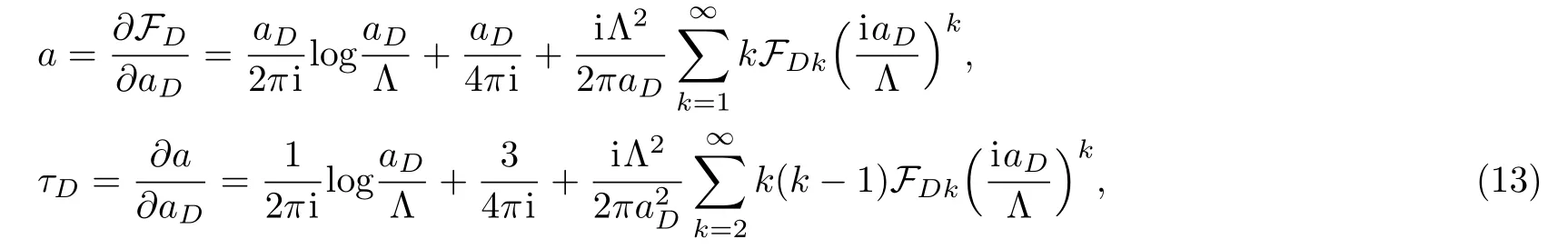
by analogy with Eq.(6)we have

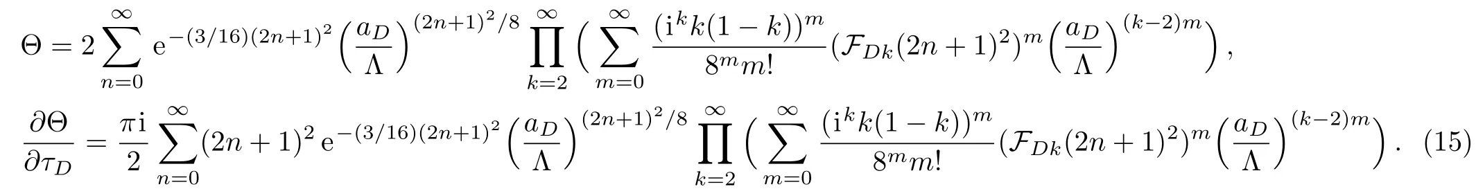
However,it should note here that from the point of view of the dual transformation,the characteristic of the theta function near the N=1 points must be replaced byα=(1/2,...,1/2)andβ=(0,...,0),at the same time,the Riemann’s theta function becomes Θ = ∑∞n=?∞exp(iπ(n+1/2)2τD),consequently it reads
We assume FD0= ?1 and that is just the outcome of normalization of the FDkif we are rescaling Λ appropriately.In this way,the prepotential FDtakes a more familiar form as that in[3]

here=iaD/Λ and taking advantage of these relations,one could derive the strong coupling expansion coefficients FDnrecursively through comparing the coefficient of the term(aD/Λ)n+1/8on both sides of the Seiberg-Witten/Whitham equation(2).
3 SU(n)Case
In this section we mainly consider the general SU(n)non-abelian supersymmetric Yang-Mills theory without doubt that the associated formulae and computations are much more complicated.To illustrate this detailedly,let us first recall that the general form of the prepotential F in the pure SU(n)supersymmetric gauge theory consists of three parts:the classical prepotential,the perturbative one-loop effects,and the k-instanton corrections,[5]namely

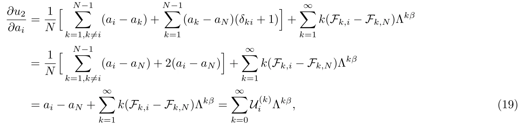
in this formalism,the derivatives of the prepotential F follow directly that

In view of the restriction to the constrain hyperplanewe should view the prepotential F(a1,...,aN)as a function of all the independent variables akexcept aNwhich results in ?i(ak?aN)= δki+1(here?imeans the partial derivative with variable ai,1≤i≤N?1).Thus we can put the RG equations in the following precise way
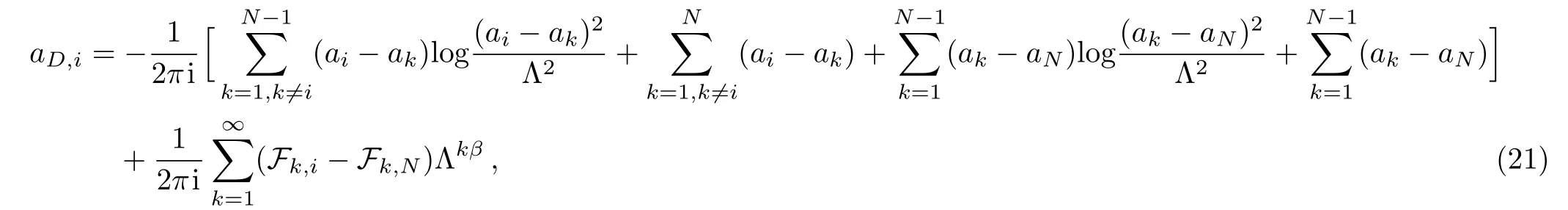
hererespectively.Now the need to pay attention to is that because of the constraint conditionthe dual variables aD,iare

and after a simple calculation we get
which leads to a fairly explicit expression for the coupling coefficients τij= ?aD,i/?aj? ?aD,i/?aN(ij)
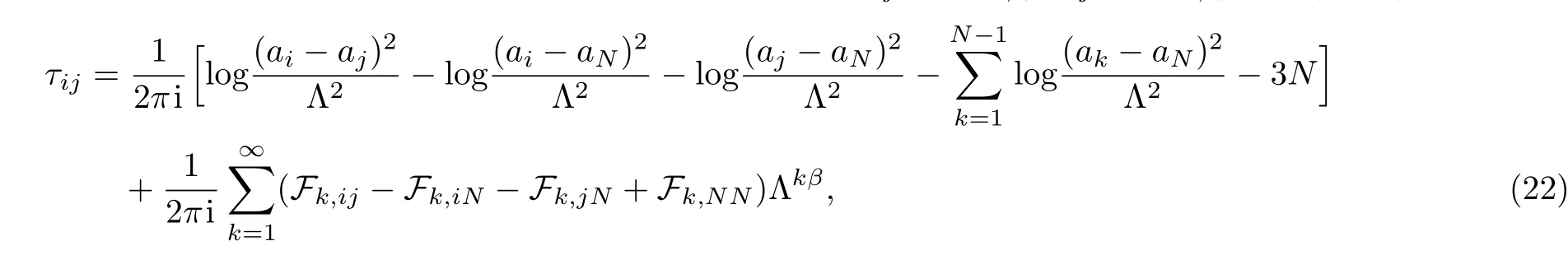
in particular,the coupling coefficients τiiare

From the previous argument we are aware of that in the general SU(n)non-abelian case,the most crucial ingredient in our analysis is the expression of Θ function.Therefore under the substitution of Eqs.(22),(23)into the de fi nition of Θ,it turns out to be
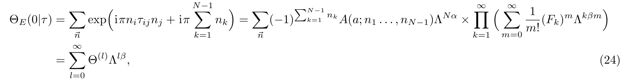
where
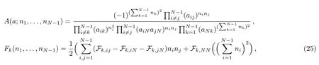
herecomes from the aNkterms in Eqs.(22)and(23).We already eliminate the e?(3/2)Nαfactor in Eq.(24)by appropriately rescaling Λ and as explained above this will be reflected in our choice for the normalization of the Fk.In addition,Θ(0)=1.Then without more efforts one is able to write down the formula for the derivative of the Θ with respect to the period matrix τijin the following form although the expressions ofare rather more involved.However,it is not difficult to prove that the indice l starts from 1,since when l=0 all integers nimust be equal to zero and from Eq.(26)we easily conclude that the coefficientsvanish.

Now let us insert the formulae of ΘE(0|τ),?τijΘE(0|τ)obtained above into Eq.(2)

which provides an exact expression for the instanton corrections coefficients

here β =2N and comparing the coefficients of powers of Λ makes it possible to compute the Fkin a purely algebraic combinatorial way

We remark here that Eq.(29)is a fundamental recursion relation for us to derive the exact n-instanton coefficient Fnby starting just from the coefficient F1through the Whitham hierarchy method in pure SU(n)supersymmetric gauge theory.As a matter of fact,the above results can even be extended to the more sophisticated situations of the massless or massive hypermultiplets included.Generally speaking,it is essentially no difficulty in applying this approach to the massless or massive hypermultiplets cases by repeating these relations(29)recursively,and after finitely many steps one is capable of getting all the correct instanton coefficients.However,in each case when k is larger,the functionsbecome much more complicated and of course the procedure of computation turns into cumbersome.Thereby for the purpose of the concrete evaluation of the Fk,one has to resort to the help of symbolic computation.In this article we basically compute 1-instanton and 2-instanton correction coefficients to illustrate the calculational procedure and then compare them with the results in paper.[5]
3.1 1-Instanton Correction
To derive the 1-instanton correction coefficient F1we consider k=1 in Eq.(29)which reads
obviously from the definition ofwe have α=2,that is

and we observe that the solutions of Eq.(31)are divided into two cases

In the first case(a),under the condition ni=1 for some i,the expression A(a;n1,...,nN?1)turns out to be

then analogous to Eq.(33)in case(b)we have

clearly,notice that when ni= ?1 and nj= ?ni=1 we find A(?i)=A(i),A(?i,j)=A(i,?j)respectively.Then recalling the coefficients

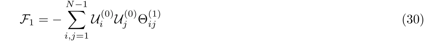
after a straightforward calculation,Eq.(30)becomes
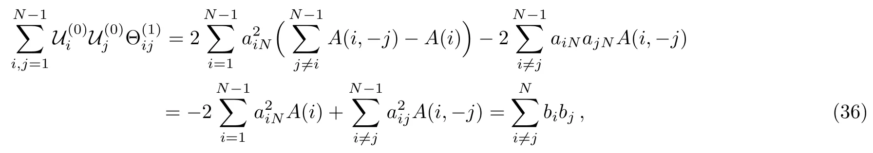
here we introduce the notationfor convenience and make use of(see the proof in Appendix A),the 1-instanton correction part of F can be written as

now if defining the functionwe can rewrite Eq.(37)in the form ofwhich is the same as the expression in Ref.[5].
3.2 2-instanton Correction
In the following section we mainly compute the 2-instant correction coefficient and we are thus led,on account of the recursion relation(29),to the F2

evidently,the calculation of F2is identical to the sum of three terms in Eq.(38)respectively.
(a)term
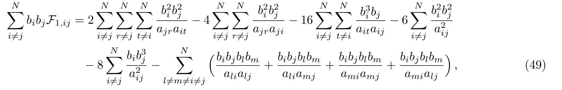
Taking into account of the definition oftogether with Eq.(35),we simplify the first term as
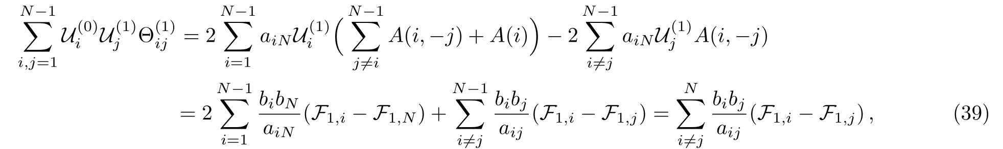
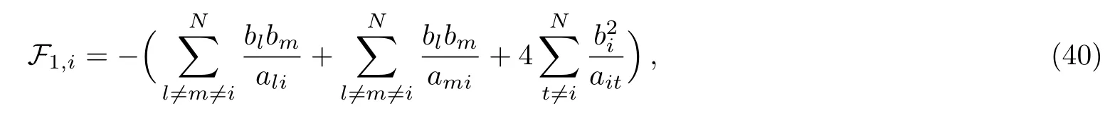
here the accurate expression of F1,i(see Appendix B)is
now utilizing Eq.(55)below,we may rewrite Eq.(39)as

(b)term
In order to obtain the explicit expression ofwe note that from Eq.(26)there are two conditions make contributions to the coefficients of Λ4N:(i) α =4,m=0;(ii) α =2,m=1,k=1.For the first condition α =4,or equivalentlywe find that the corresponding solutions are separated into two cases(we mainly consider N≥5)


thus according to the definition of Eq.(25)one obtains as well as


due to the symmetry between indices l and m,the functions of(ij)are now given by
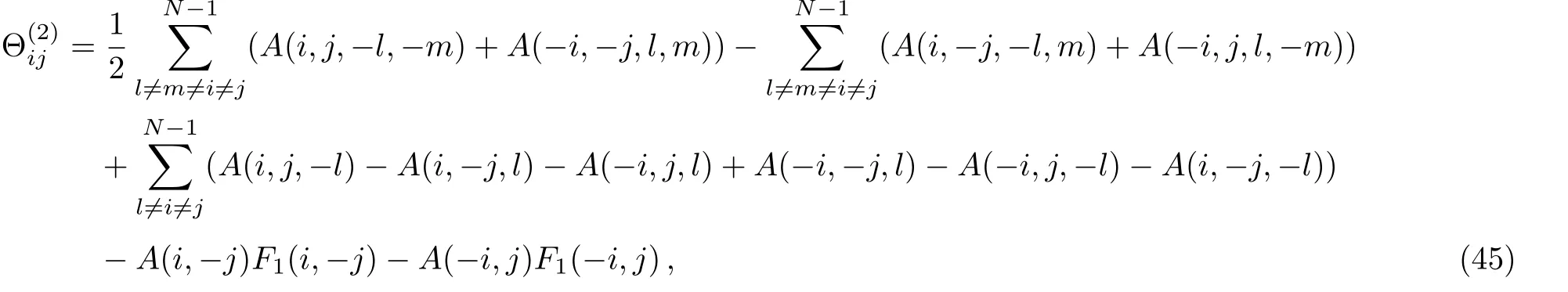
here the summation is for l,m and theare
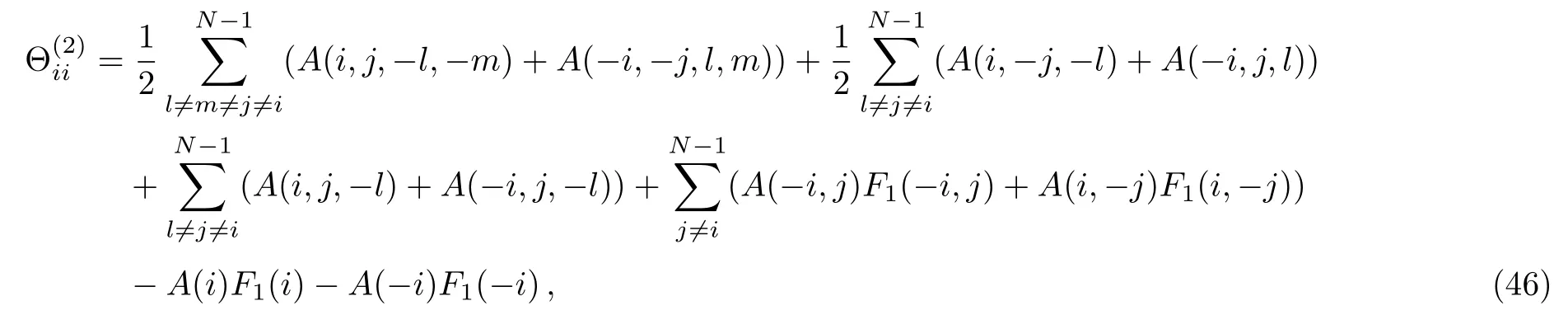
here we sum over for j,l,m.Now using these consequences and the expressions forogether with Eqs.(43),(44)above,we calculate
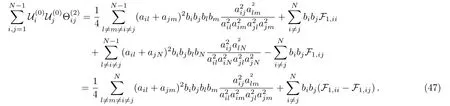
Furthermore substituting the expressionsinto Eq.(47),it is immediate to see that

and a tedious algebraic calculation of the mixed derivatives of the F1shows that
the detailed proof of Eq.(49)can be consulted in Appendix B.
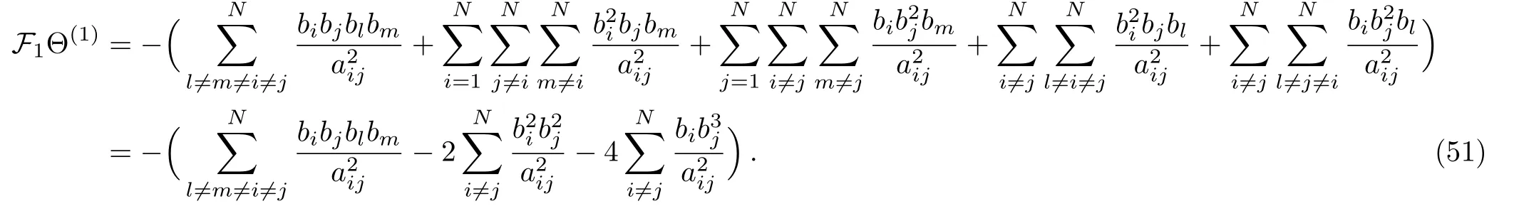
(c) F1Θ(1)term
Finally we want to compute the F1Θ(1)term and to begin with

Hence,let us combineand we have
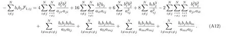
Now to proceed further it is necessary to calculate the bibjblbmterms in Eqs.(41)and(49)explicitly,actually we find

and from Appendix C,we conclude that

The above analysis enables us to derive the 2-instanton correction coefficient F2in terms of variables aijand bk.Indeed,putting all these Eqs.(41),(47)–(49)and(51)–(53)together,we therefore arrive at a more compact expression as follows

In particular,using the key relationit follows that
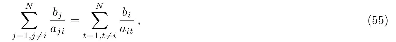
and as a consequence,various identities can now be deduced from the above Eq.(55)which will play an important role to help us simplify the expression of F2.For instance,by differentiating Eq.(55)with respect to aiand multiplyingon both sides of the result equation,then summing over for i one finds that

moreover,the similar process gives rise to

analogously let us take derivative with respect to aion both sides of Eq.(57),multiplyon the result equation and sum over for i,through a direct calculation it yields

hence inserting Eqs.(56)and(58)into(54)with the aid of Eq.(57),the computation of F2now is straightforward,and one finally obtains
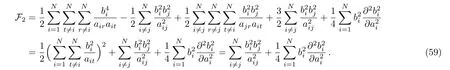
As a final comment,it is worth mentioning here that taking advantage of the notation Sk(x),the evaluation of 2-instanton correction coefficient F2can also be expanded in a more familiar form
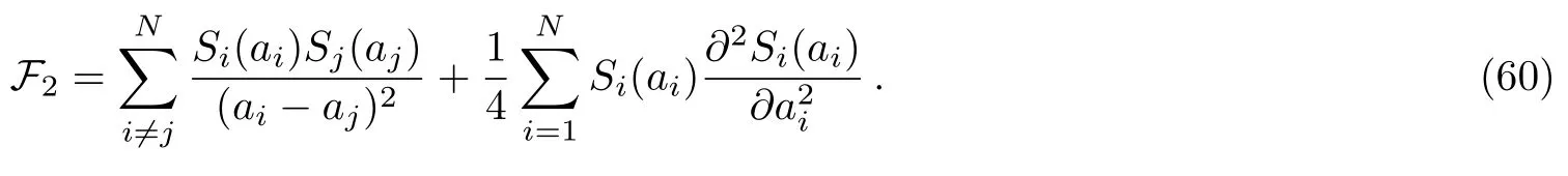
We point out here that the above expression is precisely the same as derived by E.D’Hoker,D.H.Phong and I.M.Krichever in Ref.[5].
4 Conclusion
In this paper,we primarily describe how to obtain arbitrary order instanton corrections coefficients of the effective prepotential F in N=2 pure SU(n)supersymmetric Yang-Mills theory from Whitham hierarchy and Seiberg-Witten/Whitham equations.The most important feature of this method is that there is no necessary to know the exact expressions of the Seiberg-Witten periods as functions of the moduli parameters.It is natural to generalize this idea to the other classical gauge group theory with or without hypermultiplets,which allows us to calculate the instanton corrections terms in various different Seiberg-Witten curves within a unified framework.We emphasize here that if one wants to get the recursion relations of instanton corrections coefficients from Seiberg-Witten/Whitham equations with massive or massless hypermultiplets,the number of hypermultiplets must be an even integer and the massive hypermultiplets must come up in degenerated pairs as shown in Ref.[10].Therefore it is essential to modify the formalism of the Whitham hierarchy and RG equations in order to extend our approach to the generic cases of unpaired and arbitrary masses.This would be interesting to further study.
Appendix A
For presenting the proof,it is convenient to define polynomial fand the first basic result is trivialBelow we will mostly focus on
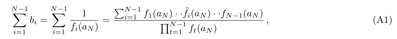
here(aN)means omitting the term fi(aN)in the products of f1(aN)··fi(aN)··fN?1(aN).Next for simplicity it is useful to introduce polynomialobviously we find gj(ak)=0 for jk,k≤N ?1,which provides

Now let us make some general considerations on the following polynomial G(x)

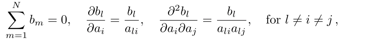
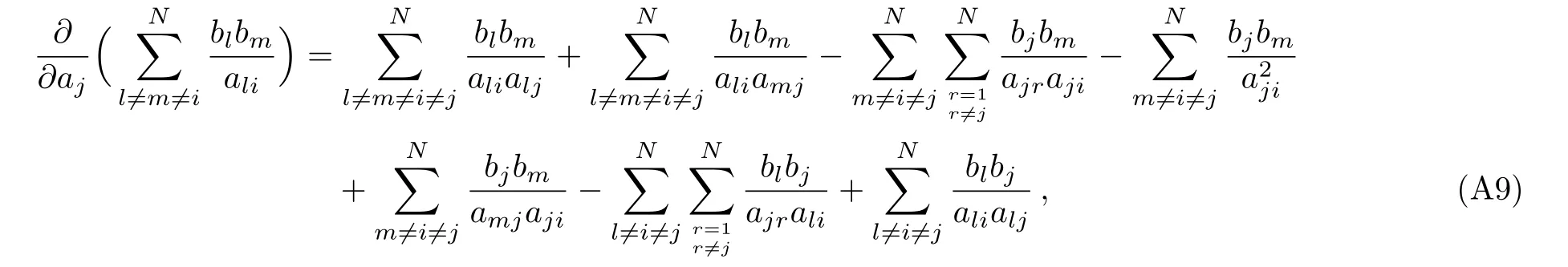
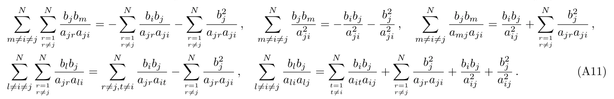
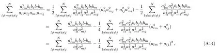
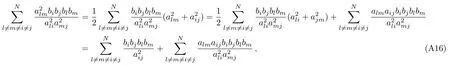
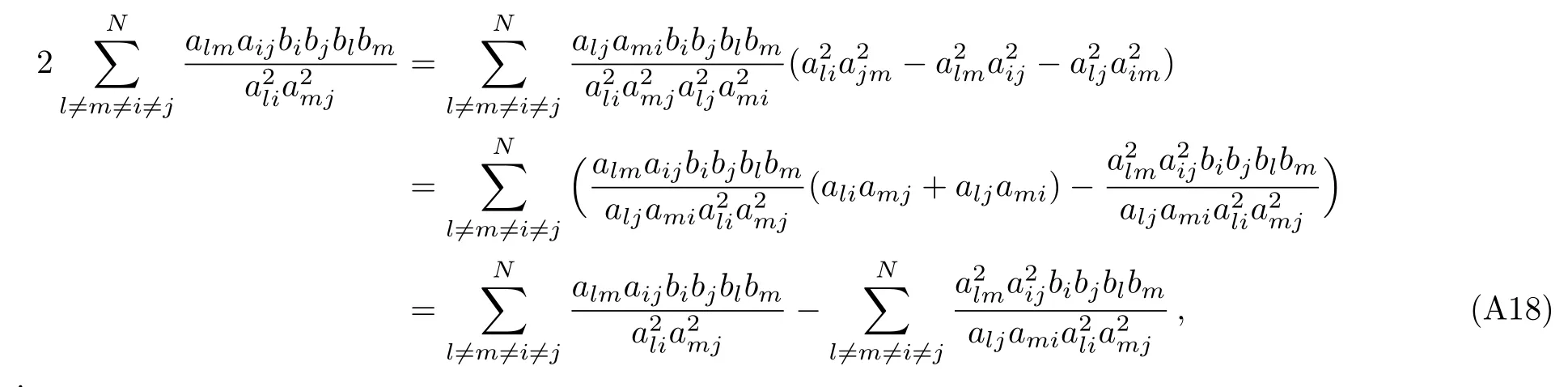
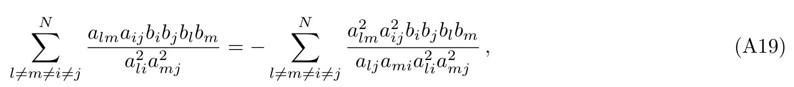
in fact,we notice that the degree of G(x)is N?2 but the polynomial has N?1 roots ai,i=1,...,N?1 which tells us that the polynomial G(x)is identically equal to zero,in other words,T(x)≡ (?1)(N?2)(N?3)/2∏N?1j on the other hand,from the definition of fi(x)we have then inserting Eqs.(A4)and(A5)into Eq.(A1),one obtains that is complete the proof. Appendix B Here we will exhibit some elementary identities about bi,which are applicable for our purpose and the corresponding proofs are straightforward According to these equations we can calculate the explicit form of F1,ij,indeed a simple and direct calculation shows that Then we give some details about how to evaluate the second derivative of Eq.(A8)with respect to the variable ajwhich can be seen as follows proceeding as before one finds(ij) Now if taking into account of Eq.(A7),we obtain a certain number of identities about the terms in Eq.(A9),these are Finally,let us substitute Eq.(A11)into(A9)together with Eq.(A10),we get Appendix C To begin with it is well known that from we have here the termsvanishing due to the antisymmetry of the indices i,j foror l,m for Analogously with the help of the equation it is enough to present that the termsvanishing because of the antisymmetry of the indices l,i or m,j for aliamj. Similarly from the identity we also have which gives rise to as explained above the first termsvanishing since the antisymmetry of the indices i,j or l,m for almaij.Now combining Eqs.(A14),(A16)with(A19)one can easily verify that [1]N.Seiberg and E.Witten,Nucl.Phys.B 426(1994)19. [2]A.Gorsky,I.Krichever,A.Marshakov,et al.,Phys.Lett.B 355(1995)466. [3]A.Klemm,W.Lerche,and S.Theisen,Int.J.Mod.Phys.A 11(1996)1929. [4]H.Itoyama and A.Morozov,Nucl.Phys.B 477(1996)855. [5]E.D’Hoker,D.H.Phong,and I.M.Krichever,Nucl.Phys.B 489(1997)179. [6]E.D’Hoker,D.H.Phong,and I.M.Krichever,Nucl.Phys.B 489(1997)211. [7]K.Ito and N.Sasakura,Nucl.Phys.B 484(1997)141. [8]J.M.Isidro,A.Mukherjee,J.P.Nunes,and H.J.Schnitzer,Nucl.Phys.B 492(1997)647. [9]M.Alishahiha,Phys.Lett.B 398(1997)100. [10]J.M.Isidro,A.Mukherjee,J.P.Nunes,and H.J.Schnitzer,Nucl.Phys.B 502(1997)363. [11]Y.Ohta,J.Math.Phys.40(1999)6292. [12]J.M.Isidro,arXiv:hep-th/0011253. [13]A.Gorsky,A.Marshakov,A.Mironov,and A.Morozov,Nucl.Phys.B 527(1998)690. [14]N.Nekrasov,Adv.Theor.Math.Phys.7(2004)831. [15]N.Nekrasov and A.Okounkov,arXiv:hep-th/0306238. [16]H.Nakajima and K.Yoshioka,Invent.Math.162(2005)313. [17]E.Martinec and N.Warner,Nucl.Phys.B 459(1995)97. [18]T.Nakatsu and K.Takasaki,Mod.Phys.Lett.A 11(1996)157. [19]E.D’Hoker and D.H.Phong,arXiv:hep-th/9903068. [20]A.Marshakov,Seiberg-Witten Theory and Integrable Systems,World Scientific,Singapore(1999). [21]A.Marshakov and N.Nekrasov,arXiv:hep-th/0612019. [22]K.Takasaki,Int.J.Mod.Phys.A 15(2000)3635. [23]K.Takasaki,Prog.Theor.Phys.Suppl.135(1999)53. [24]J.D.Edelstein and J.Mas,arXiv:hep-th/9902161. [25]J.D.Edelstein,M.G.Reino,and J.Mas,Nucl.Phys.B 561(1999)273. [26]J.D.Edelstein and J.Mas,Phys.Lett.B 452(1999)69.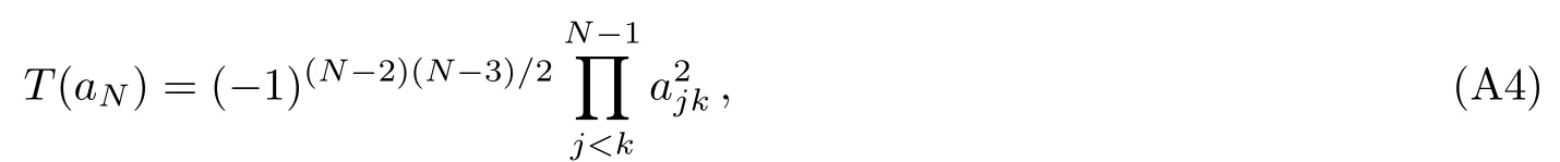


 Communications in Theoretical Physics2018年5期
- Communications in Theoretical Physics的其它文章
- Searches for Dark Matter via Mono-W Production in Inert Doublet Model at the LHC?
- Electrical Properties of an m×n Hammock Network?
- On the Generalized Heisenberg Supermagnetic Model?
- Particle Size Influence on the effective Permeability of Composite Materials?
- New Double-Periodic Soliton Solutions for the(2+1)-Dimensional Breaking Soliton Equation?
- Study on the Reduced Traffic Congestion Method Based on Dynamic Guidance Information?