Jian-Ping Wu(吳建平)and Xian-Guo Geng(耿獻(xiàn)國(guó))2School of Science,Zhengzhou University of Aeronautics,Zhengzhou 450046,China

2School of Mathematics and Statistics,Zhengzhou University,100 Kexue Road,Zhengzhou 450001,China

1 Introduction

The nonlinear Schr?dinger(NLS)equation is wellknown to be an important integrable system in mathematical physics.There are many physical contexts where the NLS equation appears.For example,the NLS equation describes the weakly nonlinear surface wave in deep water.More importantly,the NLS equation models the soliton propagation in optical fibers where only the group velocity dispersion and the self-phase modulation effects are considered.However,for ultrashort pulse in optical fibers,the effects of the third-order dispersion,the selfsteepening,and the stimulated Raman scattering should be taken into account.Due to these effects,the dynamics of the ultrashort pulses can be described by the Sasa–Satsuma higher-order nonlinear Schr?dinger equation[1?4]

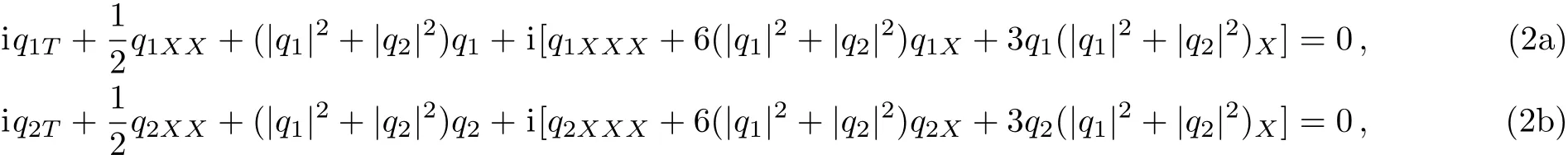
whereq=q(x,t)is a complex-valued function.Moreover,to describe the propagations of two optical pulse envelopes in birefringent fibers,some coupled Sasa–Satsuma equations were also proposed and studied.[5?9]Particularly,a coupled form of the Sasa–Satsuma equation reads[5]

whereq1=q1(X,T),q2=q2(X,T)are two complex functions of variablesX,T.As done in Ref.[5],in order to analyze Eq.(2),it is more convenient to rewrite it in the following form

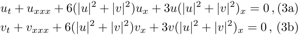
by use of the gauge,Galilean and scale transformations In this paper,we refer to Eq.(3)as the coupled Sasa–Satsuma equation.The complete integrability of Eq.(3)was established and soliton solutions were obtained using Darboux–B?cklund transformation.[5]In addition,the coupled Sasa–Satsuma equation has also been investigated via various methods such as Darboux transformation,Painlevé singularity analysis,Hirota method,[6?9]and so on.

Recently,there are many investigations on solutions of nonlinear evolution equations.[10?16]It is also known that the inverse scattering transform is a powerful approach to derive soliton solutions.However,since Eq.(3)involves a 5×5 matrix spectral problem,[5]the inverse scattering transform for this equation is rather complicated to dealwith.To our knowledge,the research in this direction has not been conducted before.The aim of the present paper is to study the multi-soliton solutions of Eq.(3)by utilizing the inverse scattering transform via Riemann–Hilbert(RH)approach.[17?25]

This paper is arranged as follows.In Sec.2,starting from the Lax pair we give direct scattering transform of Eq.(3).Then an RH problem is formulated and solved in the reflectionless cases.In Sec.3,the inverse scattering transform for Eq.(3)is established.In Sec.4,we construct multi-soliton solutions of Eq.(3).Moreover,we will give some interesting figures describing the corresponding soliton characteristics,including breather types,single-hump solitons,double-hump solitons,and two-bell solitons.

2 Riemann–Hilbert Problem

In this section,we give direct scattering transform of the coupled Sasa–Satsuma equation(3).According to Ref.[5],the Lax pair for Eq.(3)is

where Ψ = Ψ(x,t;ζ)is a column vector function of the complex spectral parameterζ,and

where

For the sake of convenience,we extend Ψ in Eq.(4)to a matrix and then introduce a new matrix spectral functionJ=J(x,t;ζ)defined by Ψ =JeiζΛx+4iζ3Λt.Then the Lax pair(4)can be rewritten as

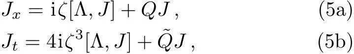
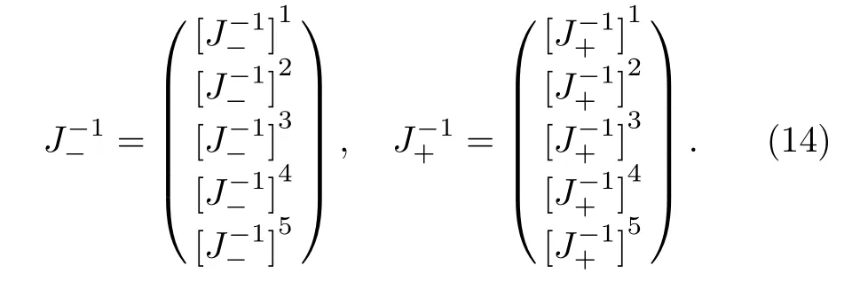
Now let us construct two matrix solutionsJ±=of Eq.(5a)under the asymptotic conditions

Here each[J±]ldenotes thel-th column ofJ±,respectively.The symbol I is the 5×5 identity matrix,and the subscripts ofJrepresent which end of thex-axis the boundary conditions are set.The matrix solutionsJ±are uniquely determined by the Volterra integral equations

It is easy to find that[J+]1,[J+]2,[J+]3,[J+]4,[J?]5allow analytic extensions to the upper halfζ-plane C+.On the other hand,[J?]1,[J?]2,[J?]3,[J?]4,[J+]5are analytically extendible to the lower halfζ-plane C?.

In what follows,we investigate the properties ofJ±.Indeed,from the fact thatQis traceless we know detJ±are independent ofx.Therefore we have detJ±=1 forζ∈ R.Moreover,J±eiζΛxare related by a scattering matrixS(ζ)=(skj)5×5

which implies that

Then it follows from the analytic property ofJ?thats55can be analytically extended to C+,whereasskj(1≤k,j≤ 4)allow analytic extensions to C?.In general,sk5,s5j(1≤k,j≤4)cannot be extended offthe realζ-axis.

Using the analytic properties ofJ±,we can construct a matrix functionP1=P1(x,ζ)which is analytic forζ∈ C+

Moreover,we have the large-ζasymptotic behavior ofP1

In order to obtain an RH problem for Eq.(3),we have to construct an analytic matrixP2in C?.To this end,we shall consider the adjoint equation of Eq.(5a)

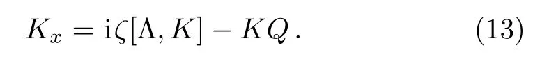
It is easy to check that the matrix inverses ofJ±satisfy Eq.(13).Let us denote

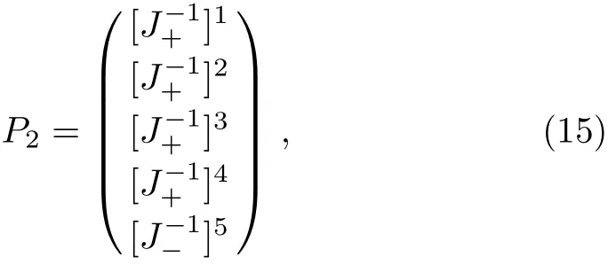
and the large-ζasymptotic behavior ofP2can be shown to be

In addition,it is easy to find thatare related by the scattering matrixR(ζ)≡ (rkj)5×5=S?1(ζ)

Moreover,similar to the scattering coeffcientsskjabove,we can show thatr55allows an analytical extension to C?,whereasrkj(1≤k,j≤4)have analytic extensions to C+.In addition,rk5,r5j(1≤k,j≤4)are only defined on the realζ-axis.

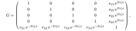
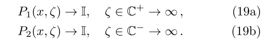
Summarizing the above results,we have constructed two matrix functionsP1andP2,which are analytic in C+and C?,respectively.Now we denote the limit ofP1from the left-hand side of the realζ-axis asP+,and the limit ofP2from the right-hand side of the realζ-axis asP?.Consequently,we obtain an RH problem for the coupled Sasa–Satsuma equation(3)

where the matrixG=G(x,ζ)is as follows

and the canonical normalization condition for this RH problem is

In order to investigate the inverse scattering transform for Eq.(3),let us solve the RH problem(18).To this end,we assume that the RH problem(18)is irregular.Here the irregularity means both detP1and detP2have certain zeros in their analytic domains.Recalling the definitions ofP1andP2,we have

To specify these zeros,we notice that there is a symmetry relation forQin Eq.(5a)

where?means the Hermitian conjugate.Therefore from Eq.(13),we get

Then it follows that

which implies the following relations

Furthermore,from the definitions ofP1andP2,the following property also holds

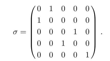
To solve the RH problem(18),we have to consider one more symmetry relation

where

From Eq.(27)we obtain that

which leads to

Obviously,Eq.(29)implies that

Furthermore,we point out that Eq.(28)also yields a property forP1itself

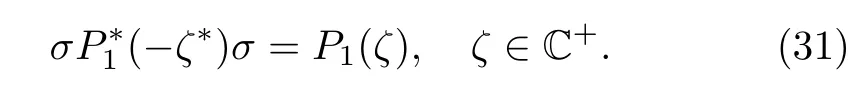
Therefore,from Eqs.(20),(21),and(25c),we find that ifζjis a zero of detP1,thenis a zero of detP2.Moreover,in view of Eq.(30c),we know thatis also a zero of detP1.Thus we can investigate the zeros of detP1in two cases.Firstly,we assume that detP1has a total number of 2Nsimple zerosζj(1 ≤j≤ 2N)satisfyingwhich are all in C+.Correspondingly,detP2possesses 2Nsimple zeros(1≤j≤2N)satisfyingwhich are all in C?.Obviously,the zeros of detP1and detP2always appear in quadruples in this case.The second case is that detP1possesses onlyNsimple zerosζj(1 ≤j≤N)in C+,where eachζjis pure imaginary.Then detP2hasNsimple zerosin C?,whereThe scattering data we need to solve the RH problem(18)consists of the continuous scattering data{s15,s35}as well as the discrete scattering data{ζj,ζj,vj,vj}.Herevjandare nonzero column and row vectors,respectively,satisfying

Next we deducevjandvjsuch that multi-soliton solutions can be obtained for the coupled Sasa–Satsuma equation(3).For the first type of zeros,we obtain a special relation by using Eqs.(26)and(32)

On the other hand,from(31)we obtain a particular column vector relation

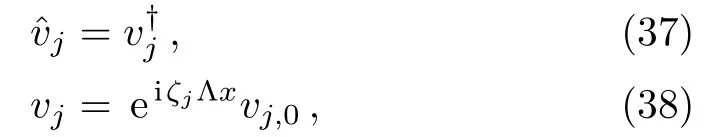
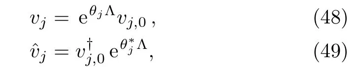
Now we shall get the vectorsvj(1≤j≤N).For this purpose,we take thex-derivative ofP1(ζj)vj=0.Then utilizing Eq.(5a),we obtain without loss of generality that

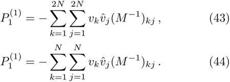
wherevj,0is independent ofx.Therefore,using Eqs.(33)–(35),all the vectorsvjandcan be determined explicitly.Note that,to derive soliton solutions for Eq.(3),we choose the matrixGin(18)to be the 5×5 identity matrix.This is guaranteed by settings15=s35=0,which corresponds to the reflectionless case.Consequently,the unique solution for the special RH problem is

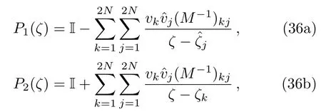
whereM=(mkj)2N×2Nis a matrix whose entries aremkj=vkvj/(ζj?ζk).For the second type of zeros,the corresponding vectorsvj,(1≤j≤N)can be derived as

wherevj,0is independent ofx.Using these vectors,the RH problem(18)in the reflectionless case can also be solved exactly

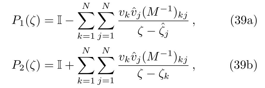
whereM=(mkj)N×Nis a matrix with entriesmkj=

3 Inverse Scattering Transform

In this section,we give the inverse scattering transform of the coupled Sasa–Satsuma equation(3),from which we recover the potentialsu,vby using the scattering data.In fact,we can expandP1(ζ)as

Then substituting it into Eq.(5a),and then comparingO(1)terms gives

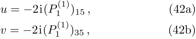
which implies thatu,vcan be obtained as

4 Multi-Soliton Solutions

To derive solutions for the coupled Sasa–Satsuma equation(3),we have to investigate the temporal evolutions of the scattering data.From(5b)and(9),and noticing the decaying properties ofuandv,we arrive at

which leads to the temporal evolutions

In addition,using Eq.(5b)we obtain thatTherefore,for the first type of zeros,we obtain

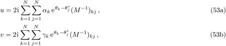
Now for the first type of zeros of detP1,we setvj,0=(αj,βj,γj,μj,1)Tto be complex constant vectors.Then utilizing Eqs.(43)and(46)–(47),from Eq.(42)we obtain anN-soliton solution formula for Eq.(3)

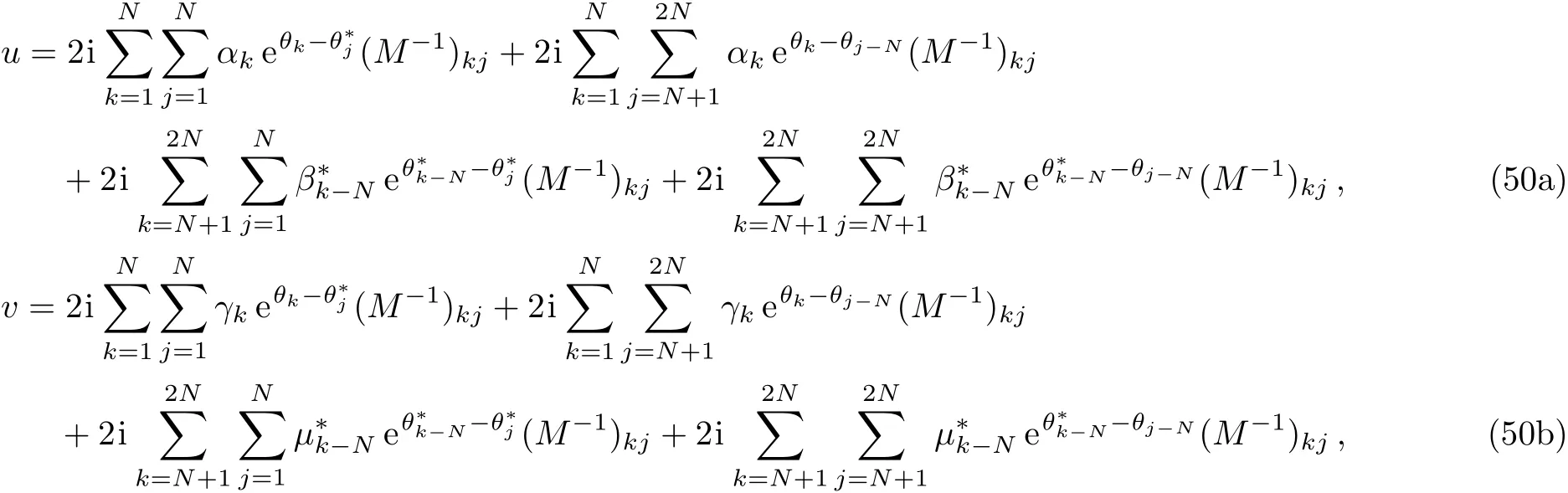
whereM=(mkj)2N×2Nwith

Now we are interested in the simplest situation that occurs whenN=1 in Eq.(50).To illustrate the single-soliton solution explicitly,we shall specify the corresponding parameters in Eq.(50).Firstly,we setβ1=α?1andμ1=γ?1in Eq.(50).Then by denotingζ1=ξ1+iη1(ξ1/=0,η1＞0),a breather-type solution for the coupled Sasa–Satsuma equation(3)is obtained from Eq.(50)

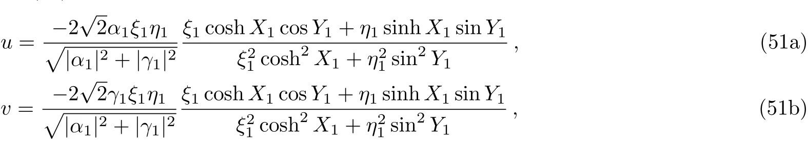
where

Its breather-type behavior is plotted in Fig.1.

Fig.1 The breather-type solution via(51) with the parameters

Secondly,we chooseβ1=μ1=0 in(50),then another type of soliton solution for the coupled Sasa–Satsuma equation(3)is obtained

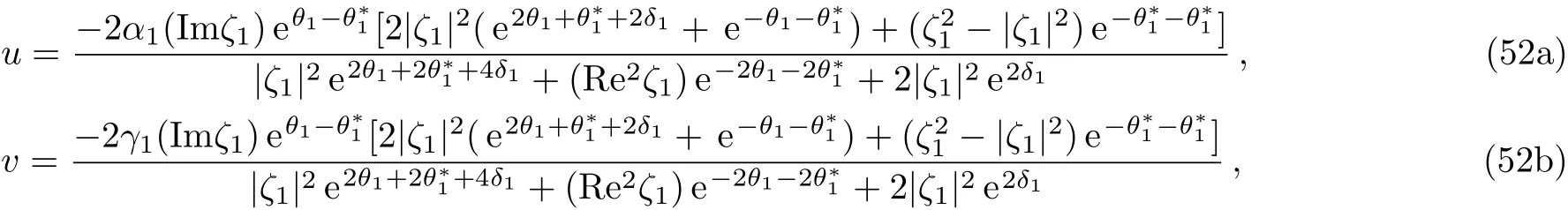
where

We remark that the single-soliton solution(52)features that it can be single-humped or double-humped,which is similar to the case for the Sasa–Satsuma equation.[1,20]By choosing appropriate parameters,we plot the single-hump and double-hump soliton solutions in Figs.2–3,respectively.

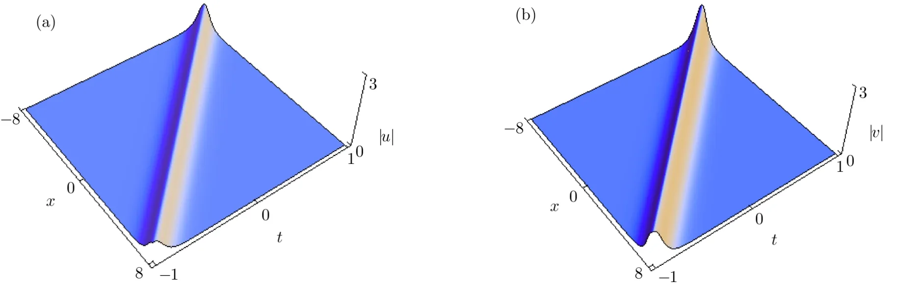
Fig.2 The single-hump soliton via Eq.(52)with the parameters

Fig.3 The double-hump soliton via Eq.(52)with the parameters

Fig.4 Collisions between two single-hump solitons via Eq.(50)with N =2,and(α1,β1,γ1,μ1)=(1,0,0,0),(α2,β2,γ2,μ2)=(1,0,1,0),ζ1=0.4+0.5i,ζ2=0.7+0.8i.

Now we shall investigate the case forN=2 in Eq.(50).To illustrate the corresponding two-soliton interactions,we first choose the parameters in Eq.(50)as(α1,β1,γ1,μ1)=(1,0,0,0),(α2,β2,γ2,μ2)=(1,0,1,0),ζ1=0.4+0.5i,ζ2=0.7+0.8i.Then a type of polarization-changing collision[2]between two single-hump solitons will be obtained.The polarization-changing collisions lead to the enhancement of intensity in one component of|u|or|v|,and the suppression of intensity in the other component,as shown in Fig.4.This figure also shows that one component of|v|even becomes zero after collision.Moreover,for the caseN=2 in Eq.(50),another type of two-soliton interaction can be obtained by choosing proper parameters.For example,we set(α1,β1,γ1,μ1)=(1,1,1,1),(α2,β2,γ2,μ2)=(1,0,2,0),ζ1=0.5+0.5i,ζ2=1+i.Under these parameters,the interactions of a single-hump soliton and a breather can be obtained,as can be seen in Fig.5.This figure demonstrates that a single-hump soliton changes into a breather when interacting with a breather.

Fig.5 Interactions between a single-hump soliton and a breather via Eq.(50)with N=2,and(α1,β1,γ1,μ1)=(1,1,1,1),(α2,β2,γ2,μ2)=(1,0,2,0),ζ1=0.5+0.5i,ζ2=1+i.

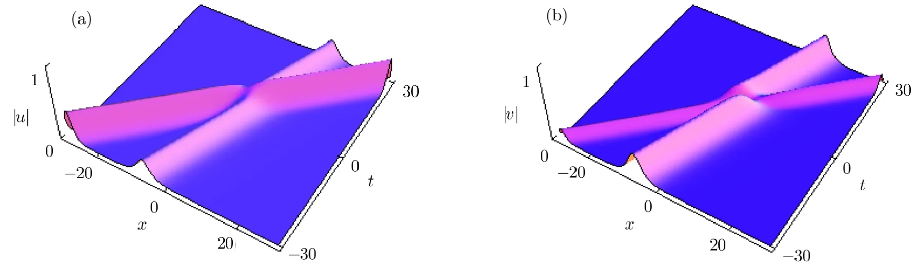
Fig.6 The two-bell soliton solution Eq.(55)with the parameters α1=1,γ1=1+i,α2=i,γ2=0.5i,ζ1=0.3i,ζ2=0.5i.

In what follows,we shall turn to the second type of zeros of detP1.In this case,we assume that detP1has onlyNsimple zerosλj(1 ≤j≤N)in C+,whereλjis pure imaginary.In this case,we obtain another kind ofN-soliton solution.Settingto be complex constant vectors,anotherN-soliton solution formula for Eq.(3)follows from(42)by using Eqs.(44),(48)–(49)

whereM=(mkj)N×Nwith

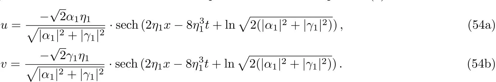
WhenN=1,Eq.(53)gives a bell-soliton solution for the coupled Sasa–Satsuma equation(3)

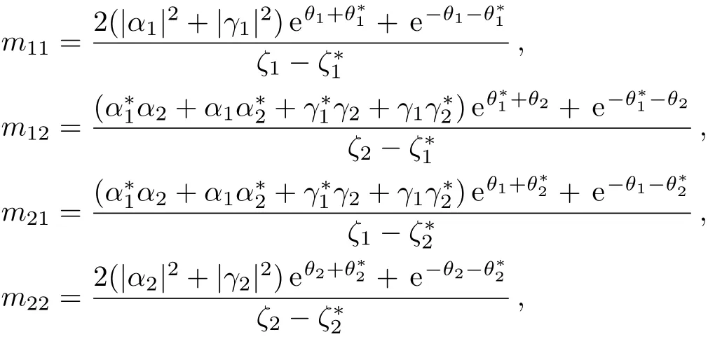
WhenN=2,Eq.(53)reduces to a two-bell soliton solution of the coupled Sasa–Satsuma equation(3)

whereM=(mkj)2×2with

5 Conclusions

In this paper,we have obtained two kinds of multisoliton solution formulae for the coupled Sasa–Satsuma equation(3).One is Eq.(50)and the other is Eq.(53).These two forms ofN-soliton solutions correspond to two different types of zero structures of the RH problem.In addition,based on the twoN-soliton solution formulae,we obtain some interesting soliton solutions which include breather-type solutions,single-hump soliton solutions,double-hump soliton solutions,and two-bell soliton solutions.

[1]N.Sasa and J.Satsuma,J.Phys.Soc.Jpn.60(1991)409.

[2]T.Xu and X.M.Xu,Phys.Rev.E 87(2013)032913.

[3]T.Xu,M.Li,and L.Li,Europhys.Lett.109(2015)30006.

[4]J.J.C.Nimmo and H.Yilmaz,J.Phys.A:Math.Theor.48(2015)425202.

[5]K.Nakkeeran,K.Porsezian,P.Shanmugha Sundaram,and A.Mahalingam,Phys.Rev.Lett.80(1998)1425.

[6]X.Lü,Commun.Nonlinear Sci.Numer.Simulat.19(2014)3969.

[7]L.C.Zhao,Z.Y.Yang,and L.M.Ling,J.Phys.Soc.Jpn.83(2014)104401.

[8]M.N.Vinoj and V.C.Kuriakose,Phys.Rev.E 62(2000)8719.

[9]A.Mahalingam and K.Porsezian,J.Phys.A:Math.Gen.35(2002)3099.

[10]M.J.Ablowitz,B.Prinari,and A.Trubatch,Discrete and Continuous Nonlinear Schr?dinger Systems,Cambridge University Press,Cambridge(2004).

[11]R.Hirota,The Direct Methods in Soliton Theory,Cambridge University Press,Cambridge(2004).

[12]X.Lü,W.X.Ma,Y.Zhou,and C.M.Khalique,Comput.Math.Appl.71(2016)1560.

[13]X.Lü,W.X.Ma,J.Yu,F.H.Lin,and C.M.Khalique,Nonlinear Dyn.82(2015)1211.

[14]X.Lü and W.X.Ma,Nonlinear Dyn.85(2016)1217.

[15]X.Lü,S.T.Chen,and W.X.Ma,Nonlinear Dyn.86(2016)523.

[16]X.Lü and L.M.Ling,Chaos 25(2015)123103.

[17]M.J.Ablowitz and A.S.Fokas,Complex Variables:Introduction and Applications,Cambridge University Press,Cambridge(2003).

[18]M.J.Ablowitz and P.A.Clarkson,Solitons,Nonlinear Evolution Equations and Inverse Scattering,Cambridge University Press,Cambridge(1991).

[19]L.D.Faddeev and L.A.Takhtajan,Hamiltonian Methods in the Theory of Solitons,Springer,Berlin(1987).

[20]J.K.Yang,Nonlinear Waves in Integrable and Nonintegrable Systems,SIAM,Philadelphia(2010).

[21]V.S.Shchesnovich and J.K.Yang,J.Math.Phys.44(2003)4604.

[22]D.S.Wang,Y.Q.Ma,and X.G.Li,Commun.Nonlinear Sci.Numer.Simulat.19(2014)3556.

[23]D.S.Wang,D.J.Zhang,and J.K.Yang,J.Math.Phys.51(2010)023510.

[24]B.L.Guo and L.M.Ling,J.Math.Phys.53(2012)073506.

[25]X.G.Geng and J.P.Wu,Wave Motion 60(2016)62.