
Slope failure simulations with MPM*
2017-06-07 08:22:46PhilipVardonBinWangMichaelHicks
水動(dòng)力學(xué)研究與進(jìn)展 B輯 2017年3期
Philip J. Vardon, Bin Wang,2, Michael A. Hicks
1. Geo-Engineering Section, Faculty of Civil Engineering and Geosciences, Delft University of Technology, Delft, The Netherlands, E-mail: p.j.vardon@tudelft.nl
2. State Key Laboratory of Geomechanics and Geotechnical Engineering, Institute of Rock and Soil Mechanics, Chinese Academy of Sciences, Wuhan 430071, China
Slope failure simulations with MPM*
Philip J. Vardon1, Bin Wang1,2, Michael A. Hicks1
1. Geo-Engineering Section, Faculty of Civil Engineering and Geosciences, Delft University of Technology, Delft, The Netherlands, E-mail: p.j.vardon@tudelft.nl
2. State Key Laboratory of Geomechanics and Geotechnical Engineering, Institute of Rock and Soil Mechanics, Chinese Academy of Sciences, Wuhan 430071, China
2017,29(3):445-451
The simulation of slope failures, including both failure initiation and development, has been modelled using the material point method (MPM). Numerical case studies involving various slope angles, heterogeneity and rainfall infiltration are presented. It is demonstrated that, by utilising a constitutive model which encompasses, in a simplified manner, both pre- and post-failure behaviour, the material point method is able to simulate commonly observed failure modes. This is a step towards being able to better quantify slope failure consequence and risk.
Heterogeneity, material point method (MPM), rainfall-induced, slope failure, strain softening
Introduction
Slope stability methods typically involve only the initial failure of the slope, although the risk from slope failure can also depend on the post-failure behaviour. For example, a superficial slide, or an initial failure which results in only a minor crest displacement, may not have a significant consequence. Conversely, a minor initial slide which triggers a larger slide, or series of slides, has a much greater consequence and therefore poses a greater risk. In this paper, a version of the material point method (MPM) has been implemented and used to investigate the failure behaviour of slopes. A series of numerical case studies, presented previously across various publications by the authors, have been examined together to illustrate the ability of MPM to simulate a number of commonly observed failure modes. In so doing, this illustrates the potential for MPM risk-based assessments involving large (e.g., post-failure) deformations, in contrast to conventional finite element methods, in which only the initial stability is often considered. A secondary objective is to summarise the work undertaken by the authors on slope failures with MPM.
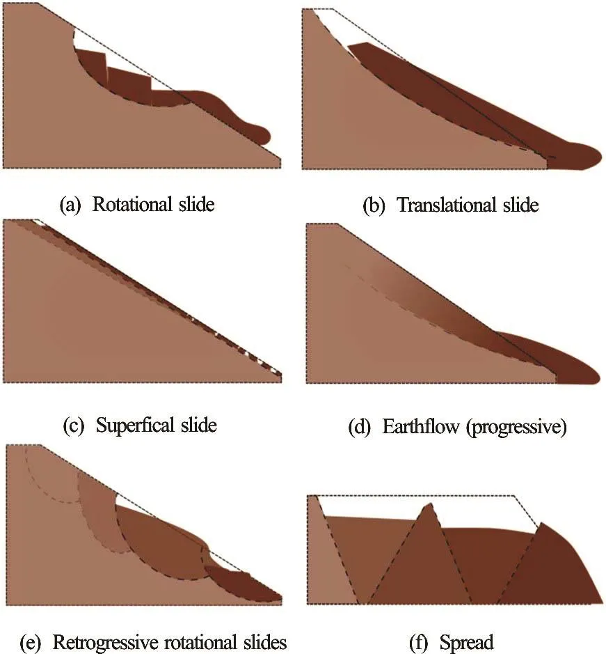
Fig.1 (Color online) Geotechnical slope failure types (after Refs.[1-4])
Several types of soil slope failure have been observed and categorised in practice[1-4], and are schematically presented in Fig.1. They include single rotational failures (Fig.1(a)), which can be small or large, large translational slides (Fig.1(b)), superficial slides(Fig.1(c)), debris or earthflows (Fig.1(d)), retrogressive rotational slides (Fig.1(e)) and spreads (Fig.1(f)). In all cases, the shear strength of the material is exceeded by the shear stress and a movement of material is observed. A variety of underlying driving mechanisms, e.g., rainfall or weathering[5], or changes in geometry, e.g., toe erosion, can trigger the failures, but it is the material behaviour during the failure which governs whether and how the initial failure progresses. In Figs.1(d), 1(e) and 1(f), the changing geometry then controls the initiation of further failures.
Typical assessment methods for slope stability include: (1) the limit equilibrium method (LEM), where a particular failure type is assumed, the geometry of the failure varied (within prescribed bounds), and the lowest ratio between the available resistance and the driving forces given as a Factor of Safety (FoS), and (2) the finite element method (FEM), or other similar numerical tools, where the material behaviour and problem geometry are characterised and the initial stability assessed, typically by reducing the strength of the material until deformations exceed a limiting value. In the first method, some knowledge of the assessed mechanism is required, although this disadvantage is at least partly offset by advantages in computational speed and conceptual simplicity. However, no insight can be gained in terms of the behaviour during the failure, displacements, or behaviour after the failure, without special treatment. FEM makes no prior assumptions regarding the failure mechanism, but, without special treatment, cannot predict the slope behaviour once the deformations have exceeded a certain limit, due to mesh tangling, hence FEM analyses often do not include features of post-failure behaviour. The material point method[6]utilises the advantages of FEM to prescribe the problem geometry, boundary conditions and material behaviour, while not prescribing failure type, but additionally facilitates the observation of the ongoing failure and final geometry by allowing the material to move through the mesh.
This paper is based on the MPM formulation presented in Ref.[7], an initial investigation of slope failures in Ref.[8], an investigation into the impact of heterogeneity in Ref.[9] and rainfall-induced slope failure in Ref.[10].
1. Methodology and material model
The main computational cycle in MPM is illustrated in Fig.2. Firstly, the state variables, e.g., velocity, acceleration, material stiffness and stress state are mapped onto the nodes of the background mesh (Fig.2(a)), secondly, a FEM analysis is undertaken, where the mesh is allowed to update its position along with the material points (using Updated Lagrangian FEM) (Fig.2(b)), and finally, the mesh is reset, with the material points remaining in their updated positions, i.e., they convect through the mesh (Fig.2(c)).
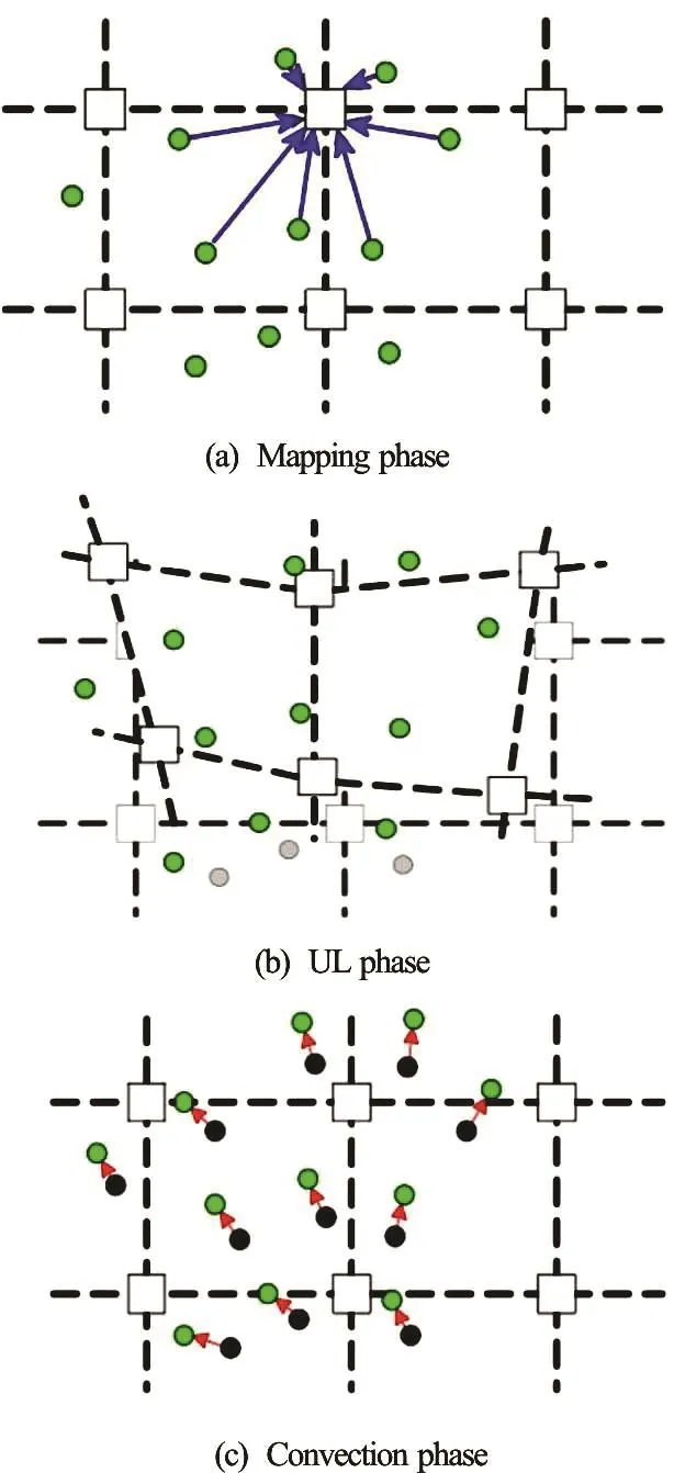
Fig.2 (Color online) The main computational phases of MPM[7]
A version of MPM has been implemented[7,10,11], in such a way that both quasi-static and dynamic analyses can be undertaken, and implicit and explicit time integration schemes chosen. In this paper only the dynamic formulation is summarized, but further details of the quasi-static formulation can be found in Ref.[11]. Where hydro-mechanical conditions prevail, a coupled hydro-mechanical version has been utilised[10], where Bishop’s stress is used to give the suction dependent strength change which reverts to effective stress at full water saturation. The formulation is specifically designed to allow for unsaturated conditions and while, in theory, it can work for saturated conditions, the numerical solution is not ideal in that case and can exhibit pore pressure oscillations.
1.1 Formulation
In all cases, at the continuum level the conservation of mass and conservation of momentum need to be satisfied. In this version of MPM, each material point has a fixed solid mass, so that the conservation of solid mass is automatically satisfied. The conservation of momentum is therefore the starting point of the formulation

where r is the mass density,vis the velocity, t is time,sis the Cauchy stress, andbis the body force due to, for example, gravity. By eliminating the lefthand term, quasi-static analyses can be undertaken.
Writing the momentum conservation (Eq.(1)) for the water yields
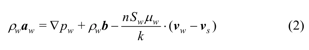
whereais the acceleration,wp is the pore pressure, n is the porosity,wS is the degree of water saturation, wm is the water viscosity, k is the soil permeability, and subscripts s and w indicate the solid and liquid phases, respectively. The last term of the equation is the force due to water flow through the material.
The momentum conservation for the mixture is also determined from Eq.(1) and can be written as

Bishop’s stress is used for the stress on the soil skeleton, with the effective stress parameter selected to be the degree of saturation. Hence

wheremis a vector allowing the pore pressure to act only isotropically and is T [1 11 0] for 2-D analyses.
It is noted that for dry conditions, or when considering total stress analyses, Eq.(3) becomes the conservation of momentum for the solid only.
The conservation of mass of water can be expressed as
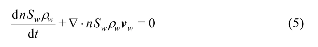
and, by including water compressibility as a material parameter, utilising the conservation of mass of the solid and assuming incompressibility of solid particles to determine the porosity change, the pore water pressure may be expressed by

where l is the rate of change of saturation with change in suction andwK is the bulk modulus of water.
1.2 Numerical implementation and solution
Typical finite element procedures are used to discretize the equations, except for utilising the material points rather than Gaussian integration points to carry out numerical integration, e.g.
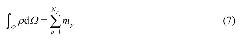
where W indicates the domain, p is a material point counter, pN is the number of material points and pm is the mass of the material point.
For the explicit formulation, the final governing equations are:
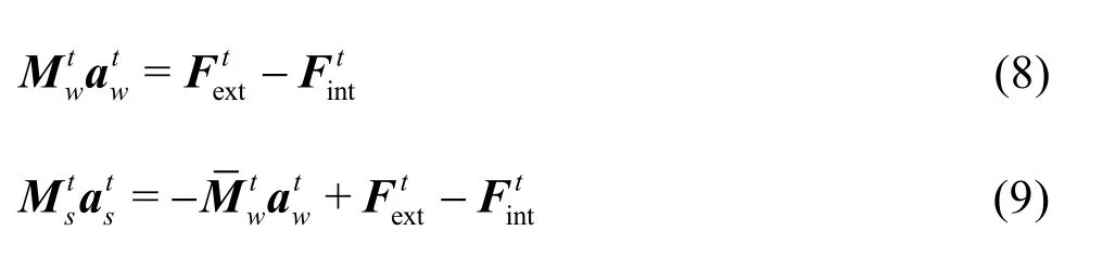
whereMis the lumped mass matrix,Fis the discretised force vector, subscripts int and ext indicate the internal and external forces, respectively, and superscript t represents time. The bar mass matrixMincludes the contributions of the porosity[11]. The external force vector includes gravitational, drag, damping and boundary forces[7,10]. The damping forces are included by using a simple damping force with a magnitude proportional to the out of balance forces, and a friction boundary condition has been implemented such that the sliding resistance is controlled by the magnitude of the normal stresses[7].
The primary variables for the solution are the accelerations of the water and solid. This is to ensure variation consistency and therefore reduce spatial oscillations in the effective stress field (and consequently other fields).
The solution algorithm comprises the following sequential steps:
(1) The accelerations of the fluid phase (Eq.(8)) are solved at the nodes.
(2) The accelerations of the solid phase (Eq.(9)) are solved at the nodes.
(3) The accelerations of the material points are updated (see subsection 1.3 below, Eq.(14)).
(4) The velocities and displacements of the material points are calculated using the explicit forward Euler method.
(5) The velocities of the nodes are updated by mapping back from the material points (Eq.(15)).
(6) The stresses and pore water pressures are updated at the material points.
For the implicit formulation, only a single phase (total stress analysis) is used herein. A large strain formulation, accounting for rate independent conditions and rotations is required[7]. The final discretised equation takes the form
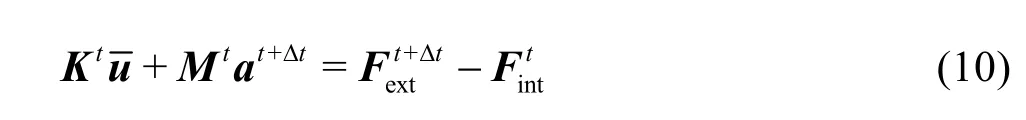
whereKis the stiffness matrix, which contains both linear (small strain) and non-linear components[7], anduis the incremental displacement. Newmark’s time integration scheme has been adopted, resulting in a modified equation with only the displacement as the primary variable
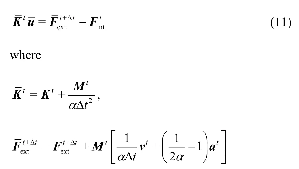
in which a is a parameter influencing the accuracy and stability of the method. In this case a= 0.25 is used, meaning that the mean acceleration is used in the time stepping.
The solution algorithm here is as follows:
(1) The displacements (Eq.(11)) are solved at the nodes.
(2) The accelerations are updated at the nodes using Newmark’s time integration scheme.
(3) The displacements and accelerations of the material points are updated using mapping.
(4) The velocities of the material points are updated (using the trapezoidal rule) based on the material point accelerations.
1.3 Mapping
Mapping is an important part of the MPM formulation. It utilises the shape functions of the finite element formulation to map between the material points and the nodes and vice versa. In general, to map nodal values to material points the following equation is used
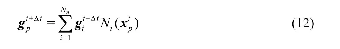
wheregis a variable, i indicates a node, p indicates a material point,nN is the number of nodes in an element,iN is the nodal shape function andxis the position of the material point.
To map between material points and nodes a similar form is taken
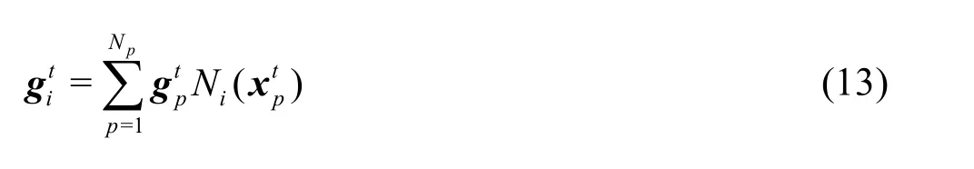
wherepN is the total number of material points in the elements connected to node i.
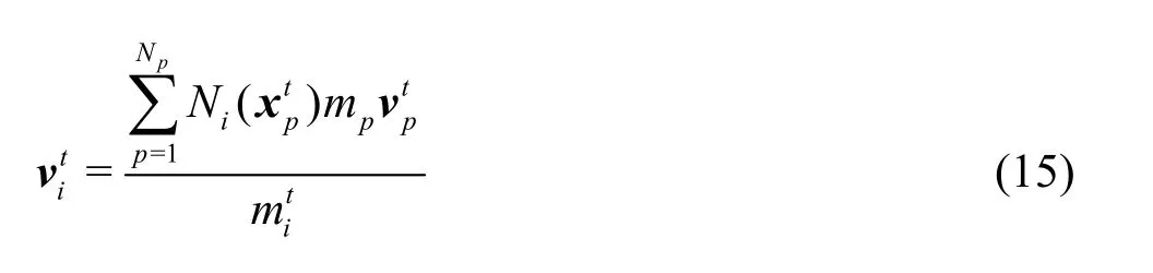
To aid the conservation laws a weighting is often needed. For example, to aid the conservation of momentum, the acceleration is mapped as follows

whereim is the mass associated with a node (determined using Eq.(13)). The velocity is also mapped ensuring the conservation of momentum
1.4 Material models
Two constitutive models have been implemented, both using simple linear elasticity prior to yield, and perfectly plastic behaviour after the ultimate (e.g., residual) strength has been reached. The first model uses the von Mises yield criterion, i.e., based on the undrained shear strength, and the second uses the Mohr-Coulomb yield criterion. For both models the postyield regime is modelled by a strain softening or hardening modulus, H, which relates changes in cohesion to the magnitude of the accumulated plastic deviatoric strain invariant. Softening behaviour (H is negative) is illustrated in Fig.3.
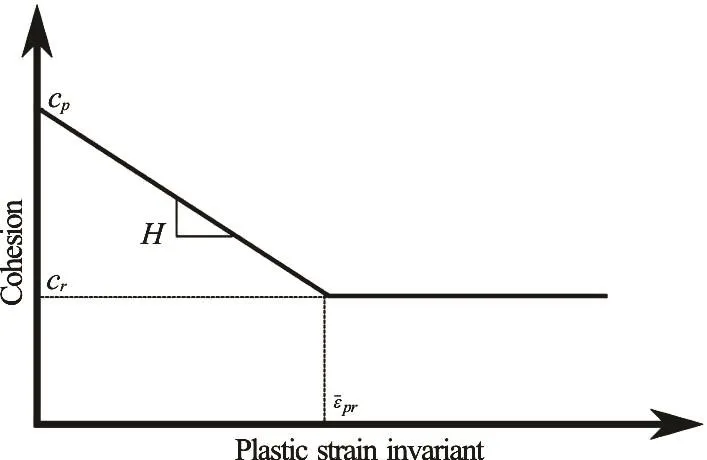
Fig.3 Schematic of the strain-softening constitutive model[7]
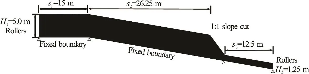
Fig.4 Numerical case study domain (not to scale)
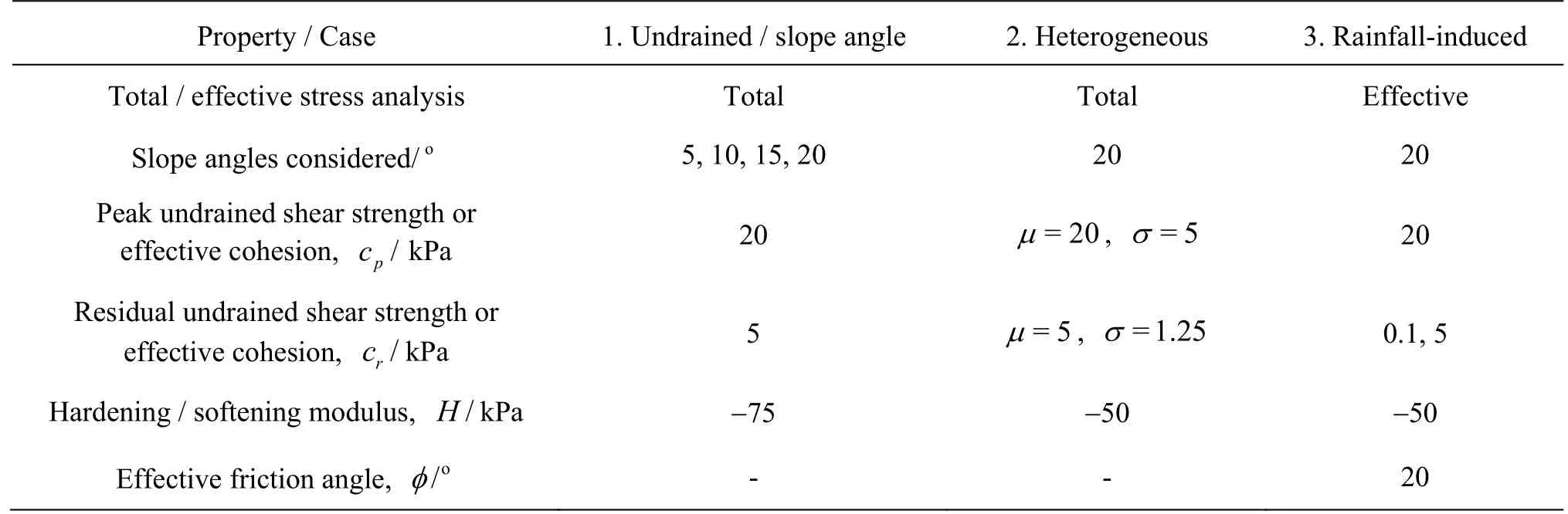
Table 1 Material properties for the case studies
To account for the spatial variability of material properties, random fields have been used and mapped directly onto the material points, i.e., each material point has a different parameter value[9]. Random fields allow the generation of statistically similar (i.e., based on the same input mean and standard deviation) independent realisations, with the spatial correlation of material properties being based on the scale of fluctuation.
2. Simulations
The case study considered here was based on a slope with a length significantly greater than the soil depth (as illustrated in Fig.4). A horizontal section of the domain was included to avoid boundary effects, as was an additional 1:1 (relative to the base of the soil layer) steeper slope, to simulate a triggering situation, e.g., toe erosion or an additional cutting. The lateral boundary conditions were rollers, allowing only vertical displacements, with the base fixed. The ground surface was free and, for hydro-mechanical simulations, the top layer of material points had a fixed value of zero pore pressure. The mesh base and sides were impermeable in the hydro-mechanical analyses.
The in situ stresses were generated in a single load step at the start of the analysis and the slope was then allowed to fail. In the total stress analyses, all of the slopes were initially unstable. In the hydro-mechanical analyses, an initial suction of 50 kPa was chosen, yielding an initially stable slope. The soil permeability and retention behaviour was selected such that, in the presence of rainfall infiltration, a sharp saturation front moves (vertically) through the soil and failure occurs quickly compared to the rate of saturation.
Three cases are presented below, with the material properties given in Table 1. The first was an undrained (total stress) analysis, with three sub-cases involving different slope angles. The second was a heterogeneous undrained analysis, with an anisotropic shear strength distribution characterised by a spatial correlation length in the horizontal direction that was 12 times larger than in the vertical direction. The third case was a rainfall-induced analysis, which considered a cohesive-frictional soil based on effective stress and two different residual cohesions.
In all analyses, prior to yield, an elastic behaviour was considered, with a Young’s modulus of 1 000 kPa and a Poisson’s ratio of 0.33. A soil volumetric weight of 20 kN/m3was considered in Cases 1 and 2, whereas a volumetric weight of 22 kN/m3was used in Case 3.
3. Results and discussion
The results for Case 1 are presented in Fig.5. In Fig.5(a), the 5oslope fails in a spread form (Fig.1(f)), where horst and graben type failure blocks can be observed. The failure is triggered by an initial rotational slide at the toe of the slope, and then moves upslope with each of the individual failures occurring separately as lateral support is removed. In Figs.5(b) and 5(c), there is also an initial rotational failure at the slope toe,which triggers a translational slide in the slope, with secondary failures occurring as the translational failure develops progressively. In Fig.5(d) two failures occur simultaneously, a small rotational failure at the toe and a large translational failure (Fig.1(b)), with the translational failure breaking up as the translation progresses downslope.
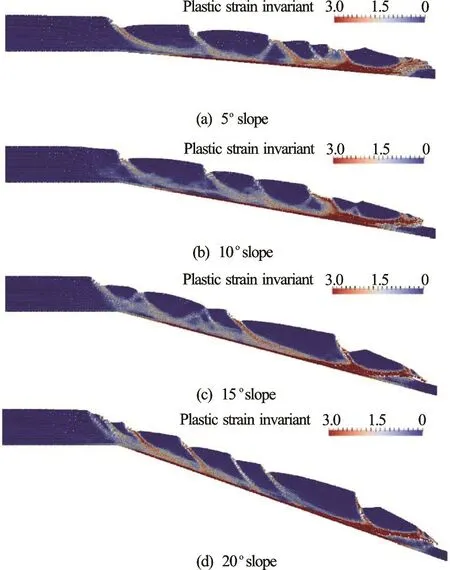
Fig.5 (Color online) Results for Case 1

Fig.6 (Color online) Results for Case 2
The results for Case 2 are shown in Fig.6. The initial peak cohesion is shown in Fig.6(a), which is also directly proportional to the residual cohesion. Figure 6(b) shows that the failure involves multiple failure zones, including one that propagates from the toe and another that propagates from mid-way up the slope. Neither of the major shear bands follows the base of the slope entirely, unlike those shown in Fig.5, due to the distribution of strong and weak zones in the soil layer. The mechanism includes a series of smaller rotational and translational failures, with rotations mainly being found at the crest and toe of the slope and multiple translational failures occurring in between.
Figure 7 shows results for pore pressure and plastic shear strain invariant for Case 3. In Figs.7(a) and 7(b), the analysis with a low residual cohesion is shown. After the initial failure is triggered, a series of failures occur, with these additional failures being both relatively superficial and occurring in a frictional manner, in an earthflow type landslide (Fig.1(d)). Eventually, almost all of the slope fails, with almost all of the possible material being incorporated into the landslide. In Figs.7(c) and 7(d), the pore pressure and plastic strain invariant are presented for the analysis with a higher residual cohesion. Again, after the initial failure a series of failures are triggered. However, these seem to be rotational (e.g., Fig.1(e)), with only a relatively small amount of material flowing as an earthflow and the run-out being significantly reduced. A final stepped situation at the upper part of the slope is seen, with an earthflow visible near the toe.

Fig.7 (Color online) Results for Case 3
Based on the landslide mechanism classification for geotechnical failures given in Fig.1, the majorityof failure types can be observed in the numerical analyses undertaken with MPM. However, it is clear that it is important to characterise the material behaviour, both pre- and post-failure, as it significantly impacts the landslide geometry and final result, e.g., the runout.
By comparing the analyses presented, a number of aspects are important for consideration in terms of quantification of the hazard. The first is that the initial failure, often characterised in FEM or LEM analyses, is often not representative of the entire failure (Figs.5 and 6) and that variability of material properties contributes significantly to the failure extent. The second is that post-failure constitutive behaviour can govern how the failure develops, e.g., the run-out, and therefore the hazard (Fig.7).
4. Conclusion
This paper presents a summary of an investigation into slope failure computation using the material point method, and compares simulated mechanisms with those observed. The series of analyses that are reported illustrate almost the full range of observed failure mechanisms. It is shown that differences in the final geometry can result, influencing the consequence and therefore the risk due to failure. The importance of characterising both the pre- and post-failure material behaviour is also demonstrated, as both have an influence on the failure mechanism.
[1] Van Asch T., Brinkhorst W., Buist H. et al. The development of landslides by retrogressive failure in varved clays [J]. Zeitschrift fur Geomorphologie, 1984, 4: 165-181.
[2] USGS. Landslide types and processes [R]. Fact Sheet 2004-3072, USGS, 2004.
[3] Varnes D. J. Slope movement types and processes (Schuster R. L., Krizek R. J. Landslides-analysis and control) [R]. Washington DC, USA: National Research Council, Transportation Research Board, Special Report 176, 1978, 11-33.
[4] Locat A., Leroueil S., Bernander S. et al. Progressive failures in eastern Canadian and Scandinavian sensitive clays [J]. Canadian Geotechnical Journal, 2011, 48(11): 1696-1712.
[5] Vardon P. J. Climatic influence on geotechnical infrastructure: A review [J]. Environmental Geotechnics, 2015, 2(3): 166-174.
[6] Sulsky D., Chen Z., Schreyer H. L. A particle method for history-dependent materials [J]. Computer Methods in Applied Mechanics and Engineering, 1994, 118(1-2): 179-196.
[7] Wang B., Vardon P. J., Hicks M. A. et al. Development of an implicit material point method for geotechnical applications [J]. Computers and Geotechnics, 2016, 71: 159-167.
[8] Wang B., Vardon P. J., Hicks M. A. Investigation of retrogressive and progressive slope failure mechanisms using the material point method [J]. Computers and Geotechnics, 2016, 78: 88-98.
[9] Wang B., Hicks M. A., Vardon P. J. Slope failure analysis using the random material point method [J]. Géotechnique Letters, 2016, 6(2): 113-118.
[10] Wang B., Vardon P. J., Hicks M. A. Preliminary analysis of rainfall-induced slope failures using the material point method [C]. Landslides and Engineered Slopes, Experience, Theory and Practice, Proceedings of the 12th International Symposium on Landslides. Naples, Italy, 2016, 2037-2042.
[11] Wang B. Slope failure analysis using the material point method [D]. Doctoral Thesis, Delft, The Netherlands: Delft University of Technology, 2017.
Acknowledgements
This work was supported by the Marie Curie Career Integration Grant (No. 333177), the “100 Talents” programme of the Chinese Academy of Science, the China Scholarship Council, and the Geo-Engineering Section of Delft University of Technology.
10.1016/S1001-6058(16)60755-2
February 16, 2017, Revised March 21, 2017)
*Biography:Philip J. Vardon, Ph. D., Assistant Professor
 水動(dòng)力學(xué)研究與進(jìn)展 B輯2017年3期
- 水動(dòng)力學(xué)研究與進(jìn)展 B輯的其它文章
- Standing wave at dropshaft inlets*
- Shedding frequency of sheet cavitation around axisymmetric body at small angles of attack*
- Numerical analysis of bubble dynamics in the diffuser of a jet pump under variable ambient pressure*
- Shock waves and water wing in slit-type energy dissipaters*
- Optimal contract wall for desired orientation of fibers and its effect on flow behavior*
- Numerical investigation of the time-resolved bubble cluster dynamics by using the interface capturing method of multiphase flow approach*