(School of Mathematics and Information Science,Henan Polytechnic University,Henan,454000,China)

§1.Introduction

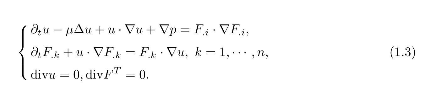
In this paper,we consider the local existence and uniqueness of strong solutions inHsfor the n-dimensional incompressible Oldroyd model:

for anyt＞0,x∈Rn,n=2,3,whereu=u(t,x)is the velocity of the flow,μ＞0 is the kinematic viscosity,pis the scalar pressure andFis the deformation tensor of the fluid.We define(▽·F)i=?jFijfor the matrixF.The Oldroyd model(1.1)describes an incompressible non-Newtonian fluid,which has the elastic properties.Many hydrodynamic behaviors of complex fluids can be regarded as consequences of the interaction between the internal elastic properties and the fluid motions.For the physical background of this model please refer to[4]and[5]for detailed discussions.

We recall the definition of the deformation tensorF.We denote byxthe Eulerian coordinate andXthe Lagrangian coordinate of a particle.It is well-known that any deformation can be described by a flow map(particle trajectory)x(t,X)for 0≤t≤T.For a given velocity fieldu(t,x),the flow mapx(t,X)is defined by the following ordinary differential equation:

To describe the dynamical processes,we define the deformation tensorIn the frame of Eulerian coordinate,we define it byF(t,x(t,X))=(t,X).After differentiating both sides of this equality with respect tot,one obtain the second equation in(1.1)2,namely,?tFij+uk?kFij=?xkuiFkjfori,j=1,2,...n,where the Einstein summation convention has been used to denote repetition index sum from 1 to n.

Assuming divF(0,x)=0,we can obtain the following equation from(1.1)2

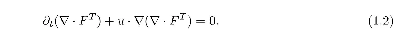
Hence,we have▽·FT=0 for anyt＞0.We denote thei-th column ofFasF.i,then▽·(FFT)=(F.i·▽)F.iby the fact▽·FT=0.Thus the system(1.1)can be rewritten in the equivalent form

Next,we recall some results for the well-posedness of the incompressible Oldroyd model.In the framework of Sobolev space,Lin,Liu and Zhang[7]established the local existence of smooth solution on either the entire space or on a periodic domain,in two dimensional case obtained the global existence of smooth solution if the initial data are sufficiently close to the equilibrium state.While Lei,Liu and Zhou[6]established the similar existence results of both local and global smooth solutions to the Cauchy problem of incompressible Oldroyd model equations in two or three dimensions provided that the initial data are sufficiently close to the equilibrium state.

Proposition 1.1For smooth initial data(u0,F0)∈H2(R2),there exists a positive timeT=T(‖u0‖H2,‖F(xiàn)0‖H2)such that the system(1.1)possesses a unique smooth solution on[0,T]with

Later,Lin and Zhang[8]proved the global well-posedness of the initial-boundary value problem of the Oldroyd model with Dirichlet conditions,when the initial data are sufficiently close to the equilibrium state.Qian[10]proved the existence and uniqueness of the local solution with initial data in critical Besov space,and if the initial data is sufficiently close to the equilibrium state in the critical Besov,the solution is globally in time.For the blow-up criteria of smooth solution to the incompressible Oldroyd model readers refer to[12]and[13].

For the non-resistive magnetohydrodynamics(MHD)equations with diffusion foruand zero resistivity for magneticB

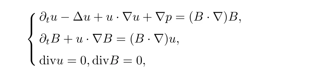
Fefferman etc.[3]obtained the local existence and uniqueness of strong solution inHsforto the MHD equations in Rn,n=2,3.The most difficult issue in demonstrating the local existence is the nonlinear term(u·▽)B.To estimate this nonlinear term,Fefferman etc.established a new commutator estimate in[3],namely,given,for▽u,B∈Hs(Rn),one has

Motivated by the work in[3],we aim at obtaining the local existence inHs,for impressible Oldroyd model(1.3)by the commutator estimate(1.1).We apply Friedrichs’method to construct a global approximate solution,then prove the approximate solution converge to the equation(1.3).Now we give our main result as follows.

Theorem 1Assumeu0,F0∈Hs(Rn)with.Then,there exists a timeT=such that equations(1.3)have a unique strong solution(u,F)withu,F∈C([0,T];Hs(Rn)).

Remark 1.1We obtain the local-in-time existence and uniqueness of strong solution inHsforto the incompressible Oldroyd model equations in Rn,n=2,3,which improves the results of[6-7].

The rest of the paper is organized as follows.In section 2,we recall briefly some definitions and lemmas which will be used in our proof.In section 3,we prove the main theorem.

§2.Preliminaries

In this preliminary section,we will present some definitions and lemmas which will be used in the proof.Throughout this paper,Cdenotes a generic positive constant which may be dependent on dimension n,the viscosity coefficientμ,but not dependent on the to-be-estimated quantity.We denote theLpnorm of a functionfby‖f‖Lp,the derivative offwith respect totbyftand the derivative with respect toxiby?i.

Fefferman etc.in[3]proved the following commutator estimate,which is crucial in the proof.

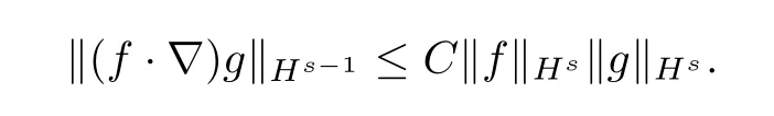
Lemma 2.1Given,there is a constantC=C(n,s)such that,for allu,Bwith▽u,B∈Hs(Rn),

To estimate the nonlinear terms,We will use the following lemma established by D.Chae in[1].

Lemma 2.2Lets＞0,p∈(1,∞),then there exists a constant C such that the following inequalities hold,

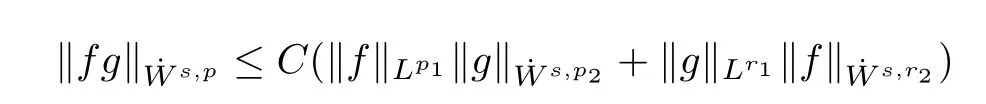
for the homogeneous Sobolev space,and

for the inhomogeneous Sobolev space,respectively,wherep1,r1∈[1,∞]such that

AsHsis an algebra,we can obtain

Lemma 2.3For fixedandf,g∈Hswith▽·f=0,we have

To prove our main theorem,We need the Picard’s theorem[9]and Lions-Aubin lemma[11].

Lemma 2.4(Picard′stheorem[9])LetAbe a Banach space andO∈Abe open set.AssumeF:O→Asatisfies the local Lipschitz condition:?X∈O,?L=L(X)andU=U(X)such that

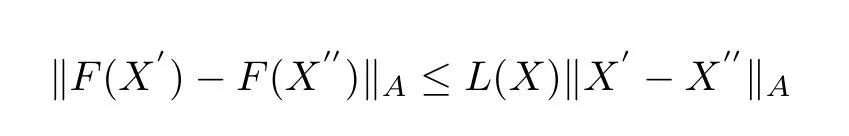
for anyX′,X′′∈U(X).Then,forX0∈U,the ODE

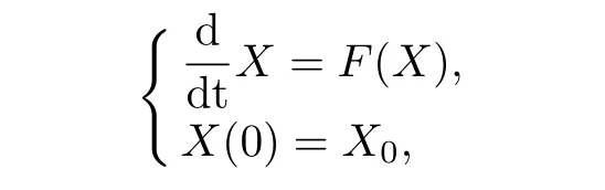
has a unique local solution,that is?T＞0 such thatX∈C1([0,T];O).In addition,eitherX=X(t)exists for all time or?T?＞0 such thatX(t)leavesOast→T?.

Lemma 2.5(Lions?Aubinlemma[11])Letq1,q2∈(1,∞)andδ2＜δ1be real number.Assume{fm}satisfies

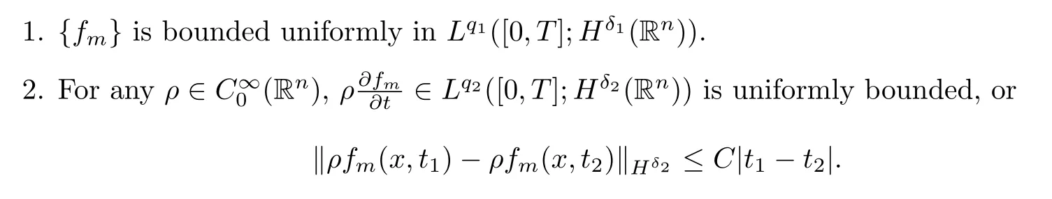
Then,there exists a subsequence offm(still denoted byfm)andf∈Lq1([0,T];Hδ1(Rn))such that,for any

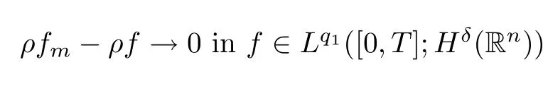
for anyδ∈(δ2,δ1).

In the proof we will use the definition of weak continuity with respective totin the functional dual spaces.

Definition 2.1we sayu∈Cw([0,T];Hm)if for any?∈H?m,

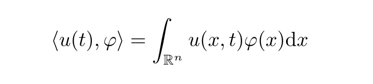
is continuous on[0,T].

At last,we introduce the truncated operatorJNand its property.

Definiton 2.2whereB(0,N)denotes the ball centered at 0 with radiusN,andχB(0,N)(ξ)is the characteristic function on B.

By virtue of the definition of operatorJNit can be easily derived the following Lemma.

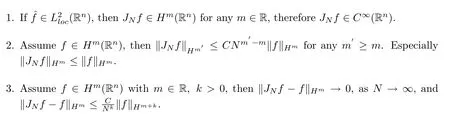
Lemma 2.6LetN≥1 be an integer.

§3.Proof of Main Results

In this section we employ the Friedrichs’method to prove Theorem 1.1.The proof is divided into five steps.

Step 1Construction of a global approximate solution.

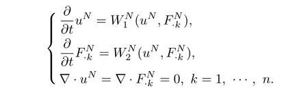
Fix an integerN＞0,assume(uN,FN)satisfies the following equations on Rn,

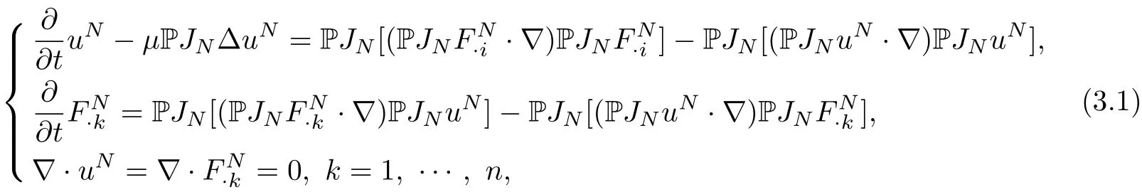
with initial dataJNu0,JNF0.Here P=δi,j+RiRjis an×nmatrix,which is the Leray projection operator onto divergence free vector fields,whereRi=?i(??)?1/2is thei?th Riesz transform.We apply the Picard theorem withA=Hs(Rn)andO=A=Hs(Rn).Then(3.1)can be rewritten in the following form

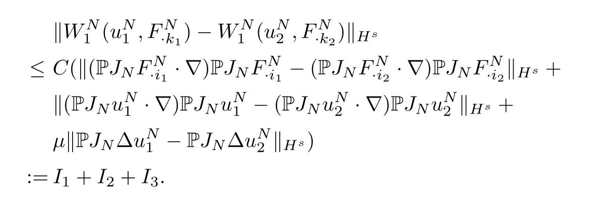
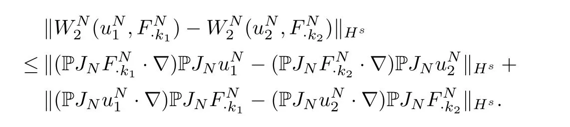
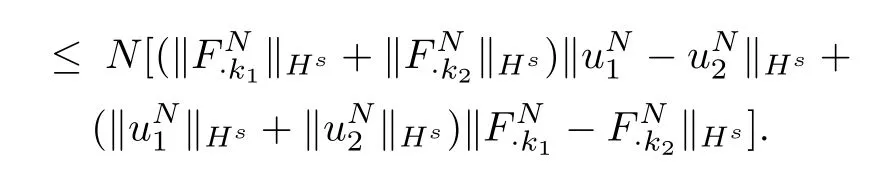
To apply the Picard’s theorem we just need to verify thatlocally Lipschitz continuous.On the one hand,

We estimateI1as follows

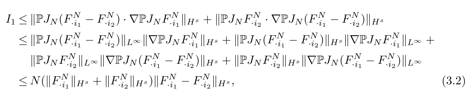
where we used the Lemma 2.2 withp=p2=r2=2 andp1=r1=∞.Similarly,we obtain

and

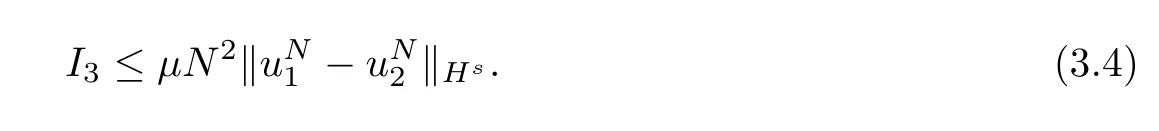
Summing up(3.2～3.4),we get

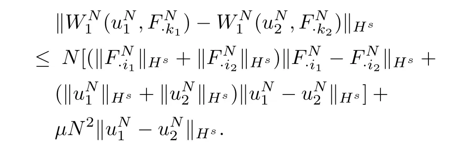
On the other hand,we also have

An argument similar to the aboveW1shows

According to the Picard theorem,we conclude that for some aT=T(N)＞0,there exists(uN,FN)∈C1([O,T];Hs),such that(uN,FN)is the unique local solution for the equation(3.1).

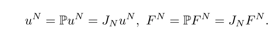
Using the properties of projection operator and truncation operator,we have P2=P,=JN.By the similar argument as before,we deduce that(PuN,PFN)and(JNuN,JNFN)also satisfy the system(3.1).By the uniqueness of the solution,we know that

Hence,the system(3.1)can be rewritten in the equivalent form

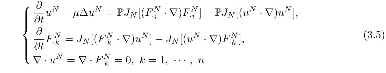
and there exists a local solution(uN,FN)to equations(3.5)for some time interval[0,T(N)].

We now prove that(uN,FN)is a global solution.TheL2energy estimate shows that

Therefore,for any timet＞0,we obtain

Then the Picard theorem implies that(uN,FN)is the global solution of(3.5).

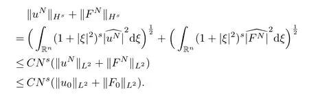
Step 2Weak convergence inHs().

are bounded uniformly inN.By the Banach-Alaoglu theorem we conclude that,for everyt∈[0,T],there exists a subsequence of(uN,FN)and(u,F)∈Hssuch that

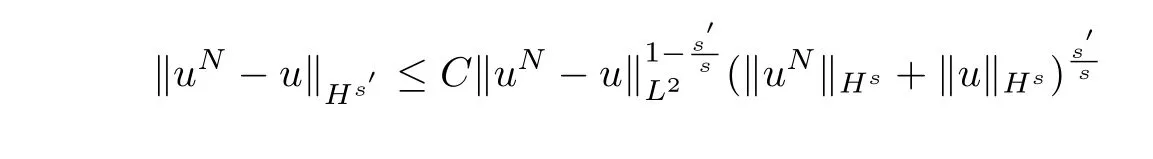
Step 3Strong convergence inHs′(s′＜s).

Now we need to verify that:for anys′＜s,(uN,FN)→(u,F)(N→∞)inHs′.By interpolation betweenL2andHs,we get:

and

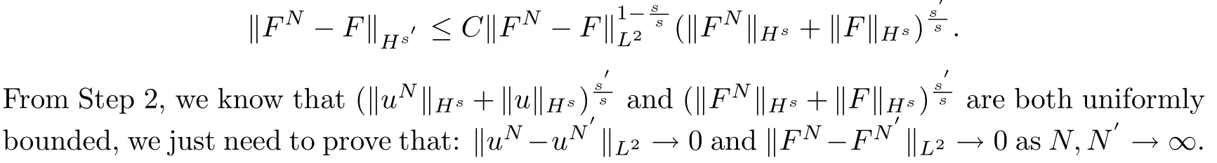
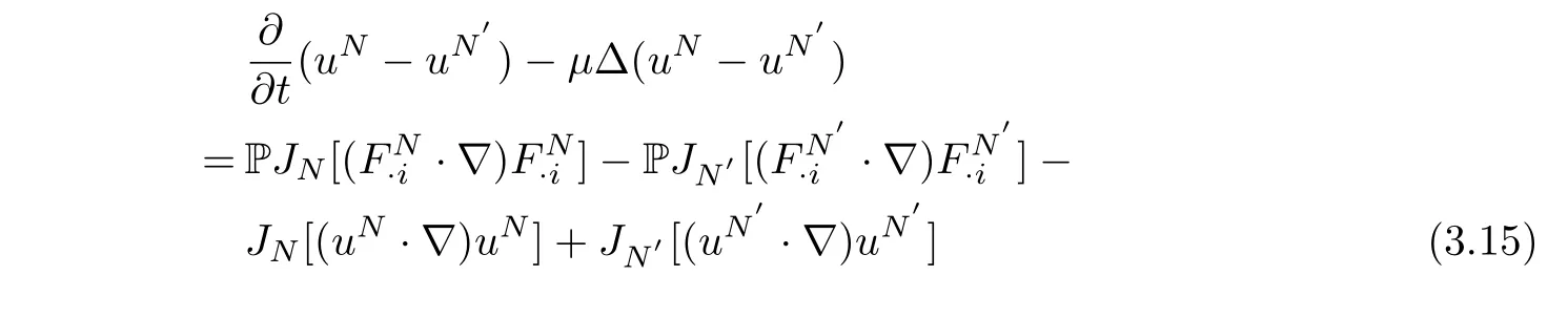
We use the method developed by Majda and Bertozzi[9]to show thatuNandFNare Cauchy sequence asN→∞.Without loss of generality,we assumeN′＞N＞0.Now,we estimate‖uN?uN′‖L2+‖F(xiàn)N?FN′‖L2.

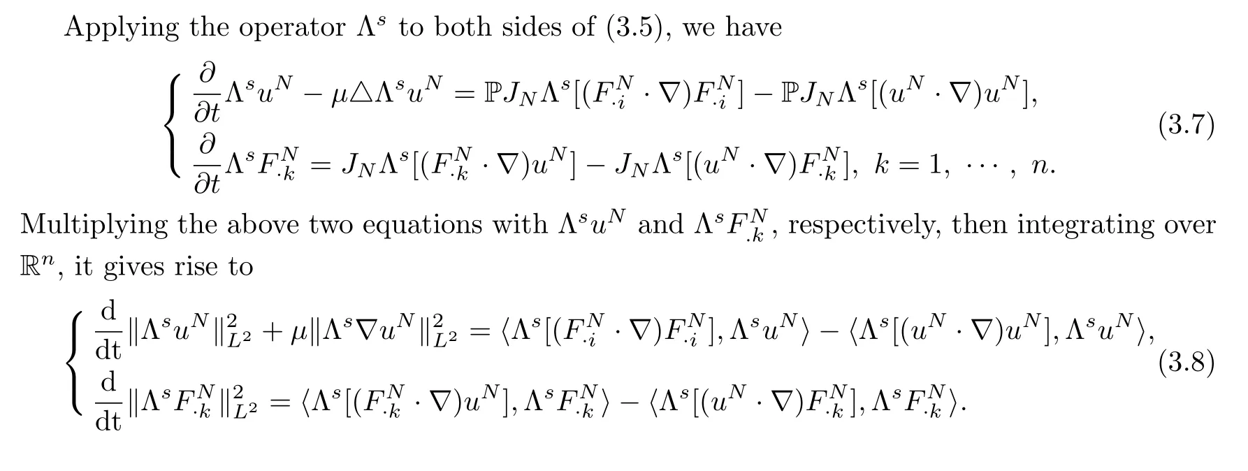
Taking the difference between the equations(3.5)forN,N′,we obtain

and

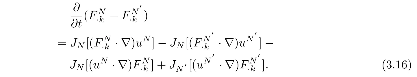
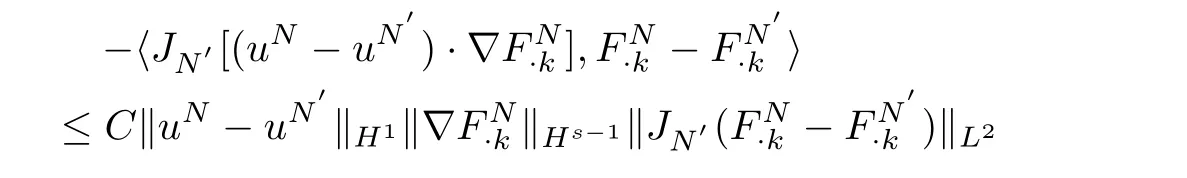
Taking theL2inner product of equation(3.15)withuN?uN′and(3.16)withrespectively,then adding them together,it follows that

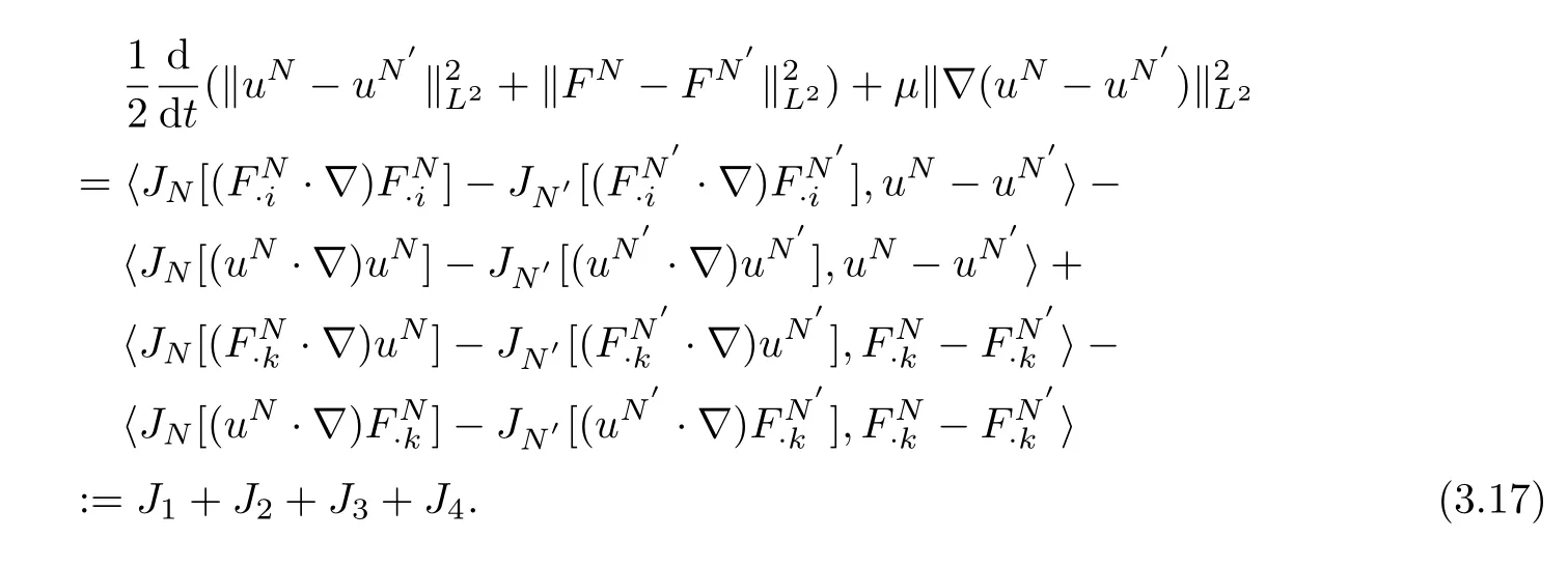
ForJ2we divide it into three parts to arrive at:

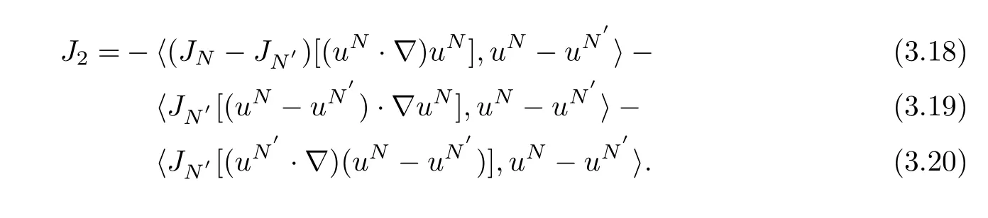
The last term(3.20)is zero by using integration by parts and the divergence-free condition.For(3.18),we apply the Lemma 2.6 to get:

with 0＜ε＜s?1.

For(3.19),we obtain

Inserting(3.21)and(3.22)intoJ2,it yields

ForJ4,we also split it into three parts,we arrive at

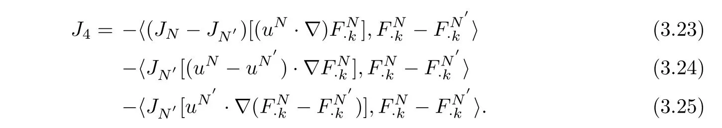
It is easy to know that the last term(3.25)is zero.

For(3.23),we handle it like(3.21)to get

with 0＜ε＜s?1.

(3.24)can be estimated by H?lder inequality and Sobolev embedding inequality in 2D and 3D cases,respectively,as Fefferman etc.did in[3].In 2D,we utilize

however,in 3D,we apply

In both cases,we obtain

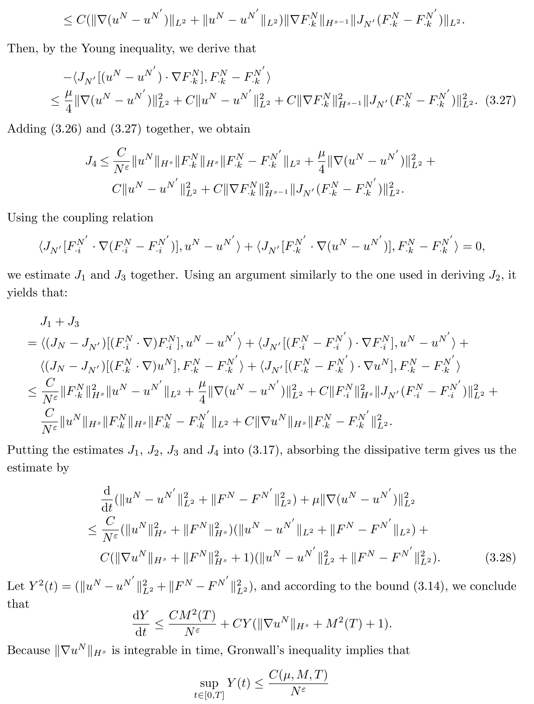
and the right-hand side goes to 0 asN→∞.

We thus have(uN,FN)→(u,F)strongly inL∞(0,T;L2(Rn)).Hence(uN,FN)→(u,F)strongly inL∞(0,T;Hs′(Rn)).

Step 4Show thatu,Fsatisfies the equations(1.3)in

We have derived that(uN,FN)→(u,F)strongly inL∞(0,T;Hs′(Rn)).By the interpolation,we can conclude that▽uN→▽ustrongly inL2(0,T;Hs′(Rn)).Thus we have△uN→△ustrongly inL2(0,T;Hs′?1(Rn)).

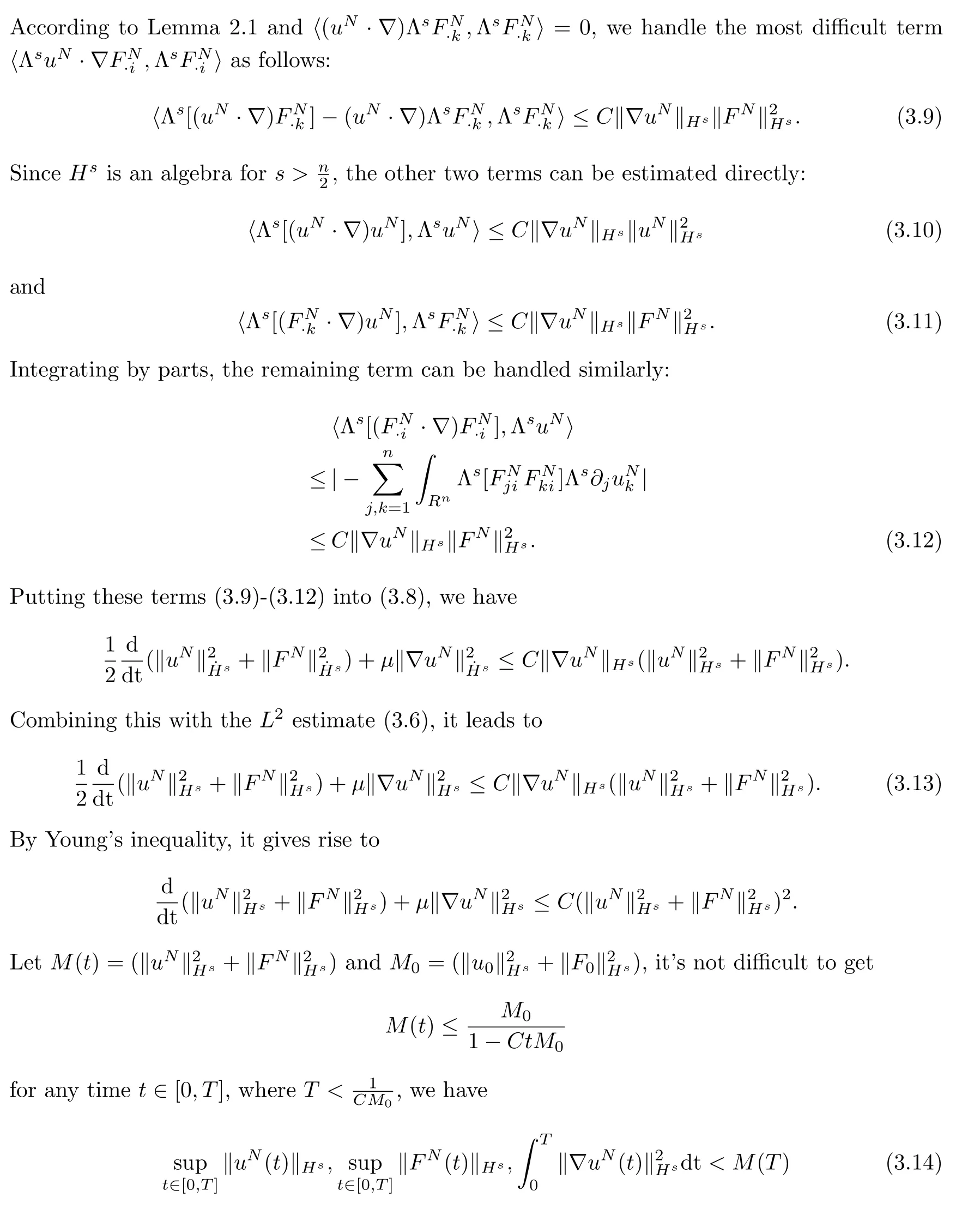
For the nonlinear term,by using the Lemma 2.3,it follows that

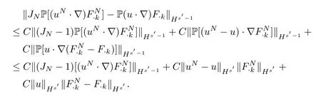
It implies that:

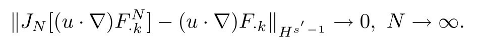
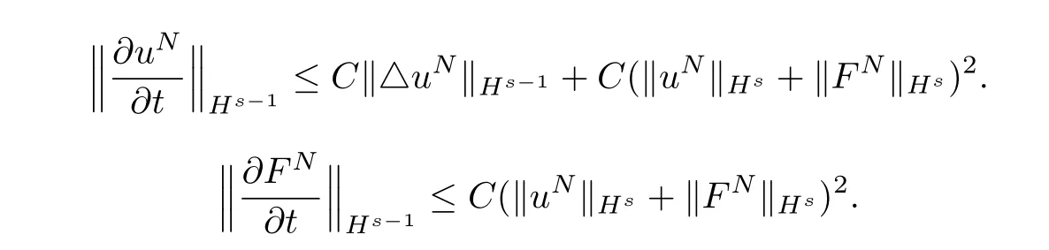
Similarly,the other nonlinear terms can be estimated in the same way.It remains to show that the time derivatives are convergence.Applying Lemma 2.3 again,we derive

The Banach-Alaoglu theorem implies that we can take a subsequenceNm→∞satisfying

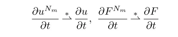
inL2(0,T;Hs?1(Rn)).Therefore(u,F)satisfies the equations(1.3)inL2(0,T;Hs′?1(Rn)).

Step 5u∈C(0,T;Hs(Rn)),F∈C(0,T;Hs(Rn)).

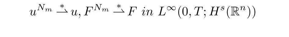
The Banach-Alaoglu theorem and the uniform bounds(3.14)guarantee the existence of the subsequence such that

and

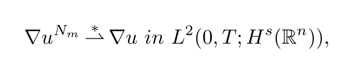
which ensures the limit satisfying

According to Theorem 4 of§5.9 in Evans[2],combiningu∈L2(0,T;Hs+1(Rn))and∈L2(0,T;Hs?1(Rn)),we deduceu∈C(0,T;Hs(Rn)).Next,we show thatF∈C(0,T;Hs(Rn)).Using the uniform bound in(3.14),we can verifyF∈CW(0,T;Hs(Rn)).It meansFis continuous in the weak topology ofHs.Hence it sufficient to prove that‖F(xiàn)‖Hs,as a function of time,is continuous.For fixedusatisfying▽u∈L2(0,T;Hs(Rn)),by an argument similar to that used in the step 2,one has

The Gronwall’s inequality implies

Then we have

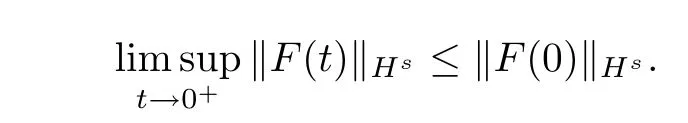
Due to the weak convergenceFN??F in Hs,asN→∞,we further haveF(t)??F(0)in Hs,ast→0+,which implies that

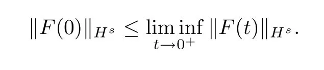
Hence,we get that‖F(xiàn)(t)‖Hsis continuous from the right at timet=0.Since theFequation is time-reversible,we obtain

Thus‖F(xiàn)(t)‖Hsis continuous at timet=0.

To prove that‖F(xiàn)(t)‖Hsis continuous at timet0∈[0,T),we consider the following system

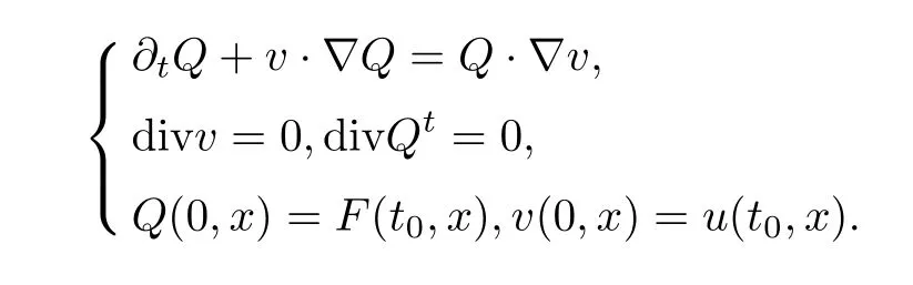
It follows that

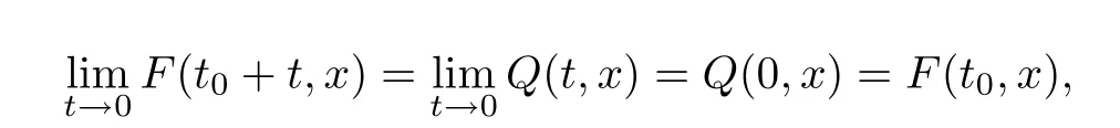
which impliesF∈C([0,T);Hs(Rn)).

The proof of uniqueness is similar to the arguments in step 3,we omit it here.We thus complete the proof of Theorem 1.1.

[1]CHAE D.On the Well-posedness of the Euler equations in the Triebel-Lizorkin spaces[J].Comm Pure Appl Math,2010,55(5):654-678.

[2]EVANS L.Partial Differential Equations[M].American Mathematical Society,Providence,Rhode Island,1998.

[3]FEFFERMAN C,MCCORMICK D,ROBINSON J,et al.Higher order commutator estimates and local existence for the non-resistive MHD equations and related models[J].J Funct Anal,2014,267(4):1035-1056.

[4]Gurtin M E,DRUGAN W J.An Introduction to Continuum Mechanics(Mathematics in Science and Engineering)[M].California:William F Ames,1981,9-76.

[5]LARSON R G.The Structure and Rheology of Complex Fluids[M].New York:Oxford University Press,1999.

[6]LEI Zhen,LIU Chun,ZHOU Yi.Global solutions for incompressible viscoelastic fluids[J].Arch Ration Mech Anal,2008,188(3):371-398.

[7]LIN Fang-hua,LIU Chun,ZHANG Ping.On hydrodynamics of viscoelastic fluids[J].Comm Pure Appl Math,2010,58(11):1437-1471.

[8]LIN Fang-hua,ZHANG Ping,On the initial-boundary value problem of the incompressible viscoelastic fluid system[J].Commun Pure Appl Math,2008,61(4):539-558.

[9]MAJDA A J,BERTOZZI A L.Vorticity and Incompressible Flow[M],Cambridge:Cambridge University Press,2002.

[10]QIAN Jian-zhen.Well-posedness in critical spaces for incompressible viscoelastic fluid system.Nonlinear Analysis.,2010,72(6):3222-3234.

[11]Simon J.Compact sets in the spaceLp(0,T;B)[J].Ann Mat Pura Appl,1986,146(1):65-96.

[12]YUAN Bao-quan.Note on the blow-up criterion of smooth solution to the incompressible viscoelastic flow[J].Discrete Contin Dyn Syst,2013,406(1):158-164.

[13]YUAN Bao-quan,LI Rui.The blow-up criteria of smooth solutions to the generalized and ideal incompressible viscoelastic flow[J].Math Methods Appl Sci,2016,38(17):4132-4139.