Nguyen Huu KHANHDepartment of Mathematics,College of Natural Sciences,Can Tho University,Vietna mE-mail:nhkhanh@ctu.edu.vnNguyen Bich HUYDepartmet of Mathematics,Ho Chi Minh University of Education,VietnamE-mail:huynb@hcmup.edu.vn

?

STABILITY ANALYSIS OF A COMPUTER VIRUS PROPAGATION MODEL WITH ANTIDOTE IN VULNERABLE SYSTEM?

Nguyen Huu KHANH?
Department of Mathematics,College of Natural Sciences,Can Tho University,Vietna m
E-mail:nhkhanh@ctu.edu.vn
Nguyen Bich HUY
Departmet of Mathematics,Ho Chi Minh University of Education,Vietnam
E-mail:huynb@hcmup.edu.vn

AbstractWe study a proposed model describing the propagation of computer virus in the network with antidote in vulnerable system.Mathematical analysis shows that dynamics of the spread of computer viruses is determined by the threshold R0.If R0≤1,the virusfree equilibrium is globally asymptotically stable,and if R0＞1,the endemic equilibrium is globally asymptotically stable.Lyapunov functional method as well as geometric approach are used for proving the global stability of equilibria.A numerical investigation is carried out to con fi rm the analytical results.Through parameter analysis,some effective strategies for eliminating viruses are suggested.

Key wordscomputer virus;virus-free equilibrium;endemic equilibrium;global stability; antidote

2010 MR Subject Classi fi cation93C15;34D23;92D30

?Received January 21,2015;revised May 13,2015.

?Corresponding author:Nguyen Huu KHANH.

1 Introduction

Several biological,social and communication systems can be described by complex networks whose nodes represent individuals,and links the interactions among them.The analysis of computer virus was the subject of interest in the field of computer science,mainly following approaches borrowed from biological epidemiology[5,21].

Models for the transmission of computer viruses based on epidemic models started to be studied by Kephart[9].He used the epidemic models to find out the rule in computer viruses and paid attention on the topological properties of the network on the spread of viruses.Many authors used the SIR and SEIR model to analyze the behavior of dynamics of computer virus[4,5,18,22].An SAIR model for computer virus,that includes an antidotal population compartment is proposed by Piqueira[19].In[23],Yang considered a computer virus model with graded cure rates.Moreover,the impact of connection mode in the computer network for thepropagation of computer virus was studied in[7,8,15].The global stability in models was determined by several approaches[11,12].Much attention was recently given to adapting biological epidemic models to real-world computer virus models under certain conditions.Muroya represented a nonresident computer virus model[17].In[6],a computer virus model in latent period was proposed.Computer virus model with nonlinear vaccination probability was studied in[3].

Previous studies for computer virus models paid more attention to high immunity of nodes.In the network,nodes(e.g.,computers)have many immunization ways such as anti-virus software,fi rewalls,virus pre-detection technology,etc.In general,anti-virus technology often follows the appearance of virus and finds the feature of virus code to create effectively and accurately defence.Because of the limitations of the current technology means,human factors,and the connection of nodes to the network,the infection of viruses in the network is problem almost impossible to avoid.One important means,that viruses in the network infected hosts,is operating system vulnerabilities[21].In the real-world system,the immunity of host to virus is dynamically variable.A computer enters the system in susceptible state,and has the immunity to all of viruses at a small rate.There are nodes which are infected are not immediately broke out and they can be in hidden state.On one hand,a infected computer can return to susceptible state by rebooting or other means,and may be re-infected.Moreover,by using effective anti-virus software one can makes a infected computer becomes immunity.For these features,antidotal technology in vulnerable system should be taken into consideration.

In this paper,we consider an improved model depicting the propagation of computer virus in the network with different antidote rates of nodes in vulnerable system,which is real-world mode for computer virus propagation.Because of reality,the latent and antivirus programs are considered.The model is given by a system of four differential equations depending on parameters.By using the method of next generation matrix[2],we find a threshold R0called basic reproduction number.In general,when R0≤1,the disease dies out and when R0＞1,the speard persists in the network.If we suppose that the endemic equilibrium also exists for R0＜1,although it is not true,then the bifurcation occurring in the model can be explained as a transcritical bifurcation.We concentrate our study on the globally stable stability of equilibria.This is obtained by Lyapunov functional approach as well as and geometric approach.A numerical investigation is carried out by Mathematica software and AUTO software package[1]con fi rming theoretical results.

The paper is organized as follows.In the next section,we introduce the structure of the transmission model,equilibria and the basic reproduction number.Section 3 deals with the local stability of equilibria.In Section 4,we prove the global stability of equilibria by using Lyapunov functional method and geometric approach.Some numerical simulations are given in Section 5.Finally,Section 6 summarizes this work.

2 The Model and its Basic Properties

2.1The Structure of the Model

We consider a propagation model of computer viruses in a network with the latent and antidotal computers.For convenience,computers are called nodes.In the real-world network,all nodes are assumed to be in one of four possible states during the virus propagation:the susceptible state(S),the latent state(L),the infectious state(I),and the recovered state(R).In state(S),the node is healthy but it can be infected by viruses.In state(L),the node is infected but the virus has not yet been triggered.In state(I),the virus has been triggered and node is infected.In state(R),the node has recovered from the non-healthy status and has immunity.The total population N(t)of computer is divided into four distinct epidemiological subgroups of individuals which are susceptible,exposed,infectious and recovered,with sizes are denoted by S(t),L(t),I(t),R(t),respectively.

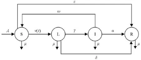
Fig.1 Transfer diagram of the model

The force of infection,v(t)=△SL(t),is the essential rate at which susceptible nodes become infected which is determined by the virus infection mode.The results based on realworld-network structure show that our network is close to P2G infection mode network,the function v(t)is expected to be L-type infection function,that is v(t)=λL(t)[7,8].

For the modeling purpose,the following hypotheses are imposed(see Fig.1):

(H1)Nodes out side the network enter the computer network with the amount A.Every node in the state(S),(L),(I)or(R)leaves the network,without connecting with others node,with the same rateμ.The total number of nodes N(t)is constant,that is N(t)=N,?t.

(H2)Every susceptible node is transferred to latent state with probability v(t)=λL(t).

(H3)Every latent node becomes infected node with constant rate γ,infected node becomes recovered node with constant rate α by using effective anti-virus program.

(H4)Each infected node returns susceptible state,by reinstall the system or other means,with constant rate ω.Latent node becomes recovered node,by using antivirus program,with constant rate δ.

(H5)Due to antidote,every susceptible node acquires temporary immunity with constant rate ε.For system vulnerability,we assume that ε＜μ.

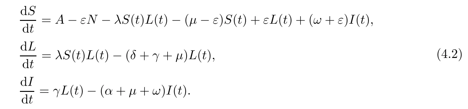
According to the above assumptions,the model is described by a system of ordinary differential equations:

with the condition S(t)+L(t)+I(t)+R(t)=N.

It follows from the system(2.1)that

2.2Equilibria

Equilibria are obtained by seting the right-hand side of the system(2.1)equals zero,then the equilibria in the coordinate(S,L,I,R)are as follows:

Endemic equilibrium P1(S?,L?,I?,R?),where S?＞0,L?＞0,I?＞0,R?＞0 and

with

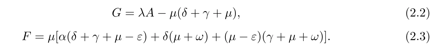
It is easy to see that the equilibrium P0always exists.Whenwe have G＞0.This implies the equilibrium P1exists for R0＞1.

2.3Basic Reproduction Number

In this section,we represent the basic reproduction number R0[2],that is the expected number of new infections from one infected individual in a fully susceptible population through the entire duration of the infectious period.The model(2.1)always has a virus-free equilibrium P0(Aμ,0,0,0).Let x=(L,I,S,R)?.Then the model(2.1)can be written as

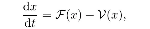
where

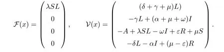
We can get

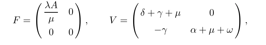
giving

The next generation matrix for the model(2.1)is

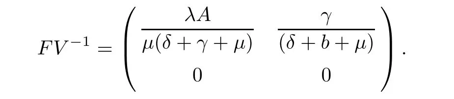
The spectral radius of matrix FV?1is ρ(FV?1)=According to Theorem 2 in[2],the basic reproduction number of the system(2.1)is

Note that when R0＞1 then G=λA?μ(δ+γ+μ)＞0 and the endemic equilibrium P1exists.

3 Local Stability and Bifurcation of Equilibria

3.1Local Stability of the Virus-free Equilibrium

Theorem 3.1P0is locally asymptotically stable if R0＜1.Whereas P0is unstable if R0＞1.

ProofThe Jacobian matrix at P0is given by

Eigenvalues of the above matrix are

Eigenvalues λ1,λ2and λ3are always negative.If R0＜1,then G＜0.It implies λ4＜0.Therefore,P0is locally asymptotically stable.Whereas,for R0＞1 then λ4＞0 and P0is unstable.

3.2Local Stability of the Endemic Equilibrium

The local stability of the endemic equilibrium P1is proved by the Routh-Hurwitz criterion.

Theorem 3.2The endemic equilibrium P1of the system(2.1)is locally asymptotically stable in ? for R0＞1.

ProofThe Jacobian matrix at P1is given by

The characteristic equation is

with

From the Routh-Hurwitz criterion,the endemic equilibrium P1is locally stable when

It is easy to see that a0＞0,a1＞0 and a3＞0.By using the Mathematica software,the conditions

3.3Bifurcation of Equilibria

The change of local stability of the equilibria P0and P1can be explained by a transcritical bifurcation.In theory bifurcation,transcritical bifurcation is a local bifurcation in which an equilibrium having an eigenvalue whose real part passes through zero.In transcritical bifurcation,an equilibrium exists for all values of a parameter and is never destroyed.Such an equilibrium interchanges its stability with another equilibrium at bifurcation value,where they collide.In our system,the virus-free equilibrium P0always exists.It is stable for R0＜1 and unstable for R0＞1.The endemic equilibrium P1exists for R1＞1 and it is unstable.If we suppose that P1also exists for R0＜1,although it is not real,then bifurcation in the model(2.1)can be seen as a form of transcritical bifurcation at R0=1.

4 Global Stability of Equilibria

This section provides the global stability of equilibria in the model.

4.1Global Stability of the Virus-free Equilibrium

We use Lyapunov function[10,14]to prove the global stability of the virus-free equilibrium.

Theorem 4.1If R0≤1,then the virus-disease equilibrium P0of the system is globally asymptotically stable in ?.

ProofWe construct the following Lyapunov function:

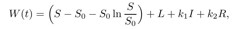
The derivative of W(t)along the solution curves of(2.1)inis given by the expression

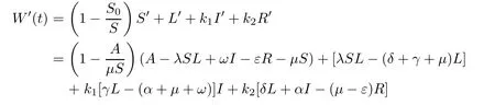
Moreover,we have

This leads to

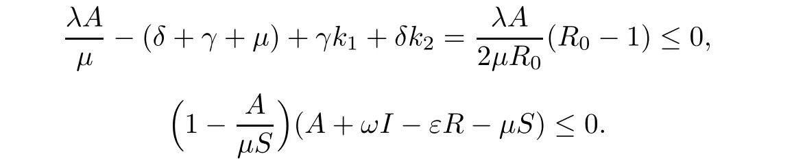
Therefore,W′(t)is negative if R0≤1.Note that,W′(t)=0 if and only ifL=I= R=0.Hence,the invariant set{(S,L,I,R)∈?:W′(t)=0}is the singleton{P0},where P0is the disease virus-equilibrium point.Therefore,by the LaSalle’s Invariance Principle[20],P0is globally stable in the set ? when R0≤1.This completes the proof.

4.2Global Stability of the Endemic Equilibrium

This section examines the global stability of the endemic equilibrium P1,for R0＞1,by using the geometric approach.First,we present some preliminaries on the geometric approach to global dynamics[12].

Consider the autonomous dynamical system:

where f:D→Rn,D?Rnopen set and simply connected and f∈C1(D).

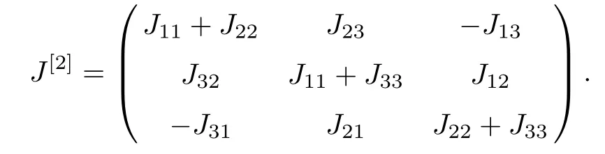
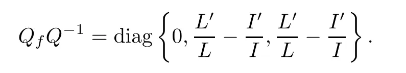
where the matrix Qfis

and J[2]is the second additive compound matrix of the Jacobian matrix J,i.e.,J(x)=Df(x).In general,for a n×n matrixmatrix and in the case n=3,we have

We will apply the following:

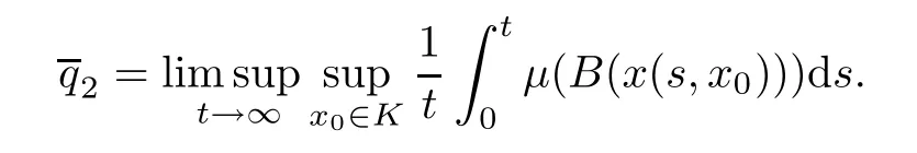
Theorem 4.2(see[12])Assume that

(H1)D1is simply connected,

(H2)There exists a compact absorbing set K?D,

(H3)The system(4.1)has a unique equilibriumin D,then the unique equilibriumof(4.1)is globally asymptotically stable in D if

Theorem 4.3For R0＞1,the system(2.1)admits an unique endemic equilibrium P1which globally asymptotically stable,provided that 2ε＜δ+γ.

ProofBecause R(t)=N?S(t)?L(t)?I(t),it is su ffi cient to consider the threedimensional system:

The Jacobian matrix of the system(4.2)is

The associated second compound matrix is given by

We set the matrix function Q by

Then

We obtain

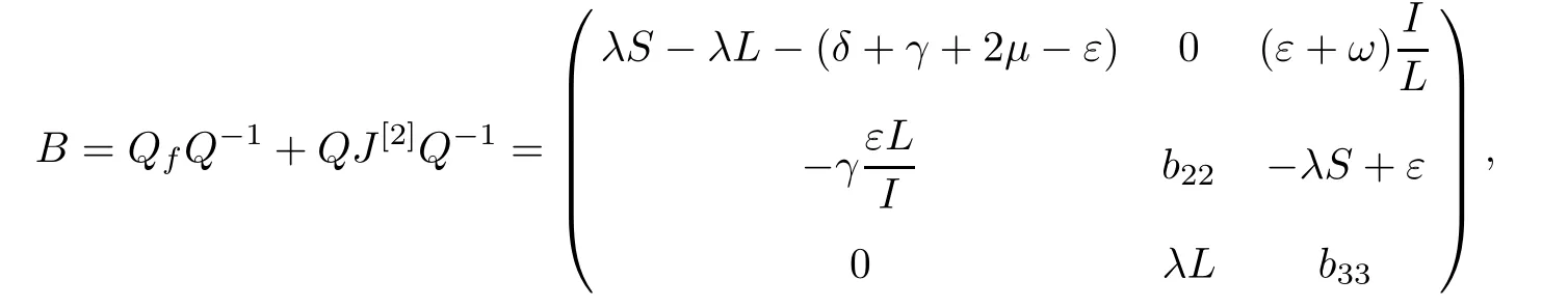
where

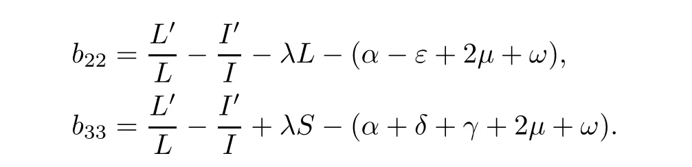
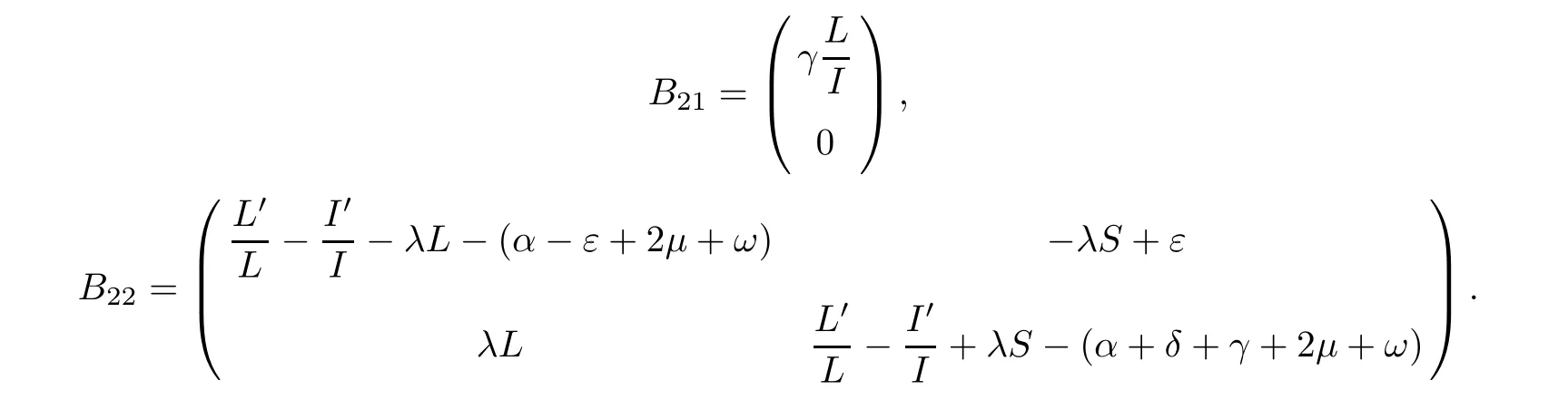
The matrix B can be written in block form

where

The vector norm|·|in R3can be chosen as

with

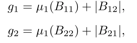
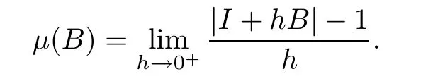
where|B12|,|B21|are matrix norms with respect to the L1vector norm andμ1denotes the Lozenski?i measure with respect to the L1norm.Speci fi cally,

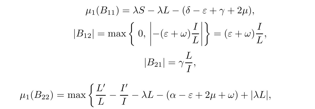
We have

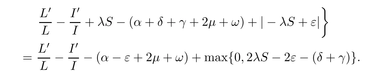
Moreover,

Based on equation

we obtain

Since S(t)is uniformly persistent,there exists T1＞0 such that S(t)≤Moreover,there also exists T2such thatfor t＞T2.Therefore,for t＞T= max{T1,T2}we haveThis implies

and

Therefore

Thus,for t＞T,we have

5 Numerical Simulation

In this section,we carry out a numerical investigation for the system(2.1)to illustrate the analytic results obtained above.Numerical results are displayed in the following fi gures.

Fig.2 shows time series of solutions of the model as R0≤1.For A=3,α=0.05,δ=0.25,ε=0.02,γ=0.001,λ=0.25,μ=0.35 and ω=0.01,we have R0=0.65784＜1.In this case,the virus-free equilibrium P0is globally asymptotically stable.With the initial condition(S(0),L(0),I(0),R(0))=(1.5,0.01,0.02,0.001),the latent component L(t)and the infectious component I(t)of solution tend to 0 as t approaches to+∞.This implies that the propagation dies out.

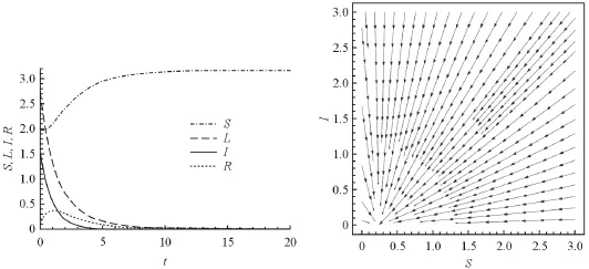
Fig.2 Time series of solutions of the model and the vector field as R0≤1

Fig.3 indicates time series of solutions of the model as R0＞1.For A=5,α=0.1,δ=0.35,ε=0.1,γ=0.45,λ=0.7,μ=0.35 and ω=0.1,we have R0=8.69565＞1.In this case,the endemic equilibrium is globally asymptotically stable.With the initial condition(S(0),L(0),I(0),R(0))=(0.5,3.5,5,5.5),the latent component L(t)tends to 3.755 and the infectious component I(t)approaches to the positive value 3.1345 as t tends to+∞.This means that the spread remains in the population.

Fig.3 Time series of solutions of the model and the vector field as R0＞1

By using AUTO software package[1],one can detect the transcritical bifurcation in the model.For A=10,α=0.35,δ=0.025,ε=0.15,γ=0.15,μ=0.35,ω=0.75 let λ vary then we get a transcritical bifurcation occurring at the value λ=2.425.The bifurcation diagram for this case is given in Fig.4.For A=10,α=0.35,δ=0.025,ε=0.025,γ=0.15,λ=0.35,ω=0.75,letμvary then a transcritical bifurcation occurs atμ=0.003.The bifurcation diagram is given in Fig.5.In Figs.4 and 5,the line passing through Solution 1,2 and 3 is the curve of virus-free equilibrium,and the line containing.Solution 4,2 and 5 is the curve of endemic equilibrium.The solid line is for stable equiliria and the dashed line is for unstable equilibria.A transcritical bifurcation occurs at Solution 2,corresponding to R0=1.We also obtain the same bifurcation when other parameters vary.

Fig.4 Bifurcation of the model as λ varies

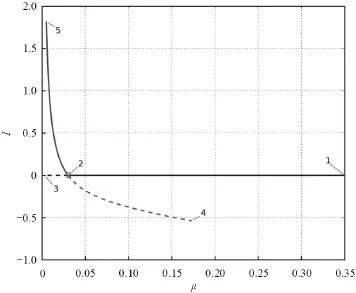
Fig.5 Bifurcation of the model asμvaries

6 Conclusions

In this paper,an improved model for propagation of computer virus in the network,that containing the latent,antidotal computers and susceptible computers with low cure rate,is introduced and studied.The basic reproduction number R0is the threshold condition that determines the propagation dynamics.When R0≤1,the system has only a virus-free equilibrium P0which is globally asymptotically stable.It implies that the propagation is extinct eventually.When R0＞1,the system has a unique endemic equilibrium P1,which is globally asymptotically stable.This shows that the transmission persists in the network and tends to a positive steady state.As results indicate that spread of computer virus is very sensitive to contact parameter λ,and transform parameters δ,α,ω andμ.The propagation will slow down if the value of λ is decreasing,and δ,α,ω andμare increasing(see Figs.4 and 5).This showsthe way to reduce the spread of computer viruses in the network.

References

[1]Doedel E J,Pa ff enroth R C,Champneys A R,Fairgrieve T F,Kuznetsov Y A,Sandstede B,Wang X.Continouation and bifurcation software for ordinary di ff eential equations.http://sourceforge.net/projects/auto2000/

[2]Driessche P,Watmough J.Reproduction numbers and sub-threshold endemic equilibria for compartmental models of disease transmission.Math Biosci,2002,180:29-48

[3]Gan C,Yang X,Liu W,Zhu Q.A propagation model of computer virus with nonlinear vaccination probability.Commun Nonlinear Sci,2014,19(1):92-100

[4]Grassberger P.Critical behavior of the general epidemic process and dynamical percolation.Math Biosci,2002,66(3):35-101

[5]Han X,Tan Q.Dynamical behavior of computer virus on Internet.Appl Math Comput,2010,217:2520-2526

[6]Hu Z,Wang H,Liao F,Ma W.Stability analysis of a computer virus model in latent period.Chaos Soliton Fract,2015,75:20-28

[7]Yuan H,Chen G.Network virus-epidemic model with the point-to-group information propagation.Appl Math Comput,2008,206:357-367

[8]Hua Y,Junjie W,Guoquing C.Infection function for virus propagation in computer network:An empirical study.Tsingchua Science and Technology,2009,14(5):669-676

[9]Kephart J O,White S R,Chess D M.Computers and epidemiology.IEEE Spectrum,1993,30:20-26

[10]Korobeinikov A.Lyapunov functions and global properties for SEIR and SEIS epidemic models.Math Med Biol,2004,21:75-83

[11]Li M Y,Muldowney J S.Global stability for the SEIR model in epidemiology.Math Biosci,1995,125:155-64

[12]Li M Y,Muldowney J.A geometric approach to global stability problems.SIAM J Math Anal,1996,27(4):1070-1083

[13]Li J,Xiao Y,Zhang F,Yang Y.An algebraic approach to proving the global stability of a class of epidemic models.Nonlinear Anal Real World Appl,2012,13:2006-2016

[14]Lyapunov A M.The General Problem of the Stability of Motion.London:Taylor and Francis,1992

[15]Ma C,Yang Y,Guo X,Improved SEIR viruses propagation model and the patch’s impact on the propagation of the virus.J Comput Inform Sys,2013,9(8):3243-3251

[16]Martin R H.Logarithmic norms and projections applied to linear different differential systems.J Math Anal Appl,1974,45:432-454

[17]Muroya Y,Li H,Kuniya T.On global stability of a nonresident computer virus model.Acta Math Sci,2014,34(5):1427-1445

[18]Ren J G,Yang X F,Zhu Q Y,Yang L X,Zhang C M.A novel computer virus model and its dynamics.Chaos Soliton Fract,2012,45:74-79

[19]Piqueira J R C,Araujo V O.A modi fied epidemiological model for computer viruses.Appl Math Comput,2009,213:355-360

[20]Salle J P.The Stability of Dynamical System.Philadelphia,PA:SIAM,1976

[21]Serazzi G,Zanero S.Computer virus propagation models.Lecture Notes in Computer Science,2004,2965:26-50

[22]Zhu Q,Yang X,Ren J.Modeling and analysis of the spread of computer virus.Commun Nonlinear Sci Numer Simulat,2012,17:5117-5124

[23]Yang L X,Yang X,Zhu Q,Wen L.A computer virus model with graded cure rates.Nonlinear Anal-Real,2013,14:414-422

[24]Yuan H,Chen G.Network virus-epidemic model with the point-to-group information propagation.Appl Math Comput,2008,206:357-367