Shenquan Wang , Wenchengyu Ji , Yulian Jiang , Yanzheng Zhu ,,, and Jian Sun ,,

Abstract—This paper develops a quadratic function convex approximation approach to deal with the negative definite problem of the quadratic function induced by stability analysis of linear systems with time-varying delays.By introducing two adjustable parameters and two free variables, a novel convex function greater than or equal to the quadratic function is constructed, regardless of the sign of the coefficient in the quadratic term.The developed lemma can also be degenerated into the existing quadratic function negative-determination (QFND)lemma and relaxed QFND lemma respectively, by setting two adjustable parameters and two free variables as some particular values.Moreover, for a linear system with time-varying delays, a relaxed stability criterion is established via our developed lemma,together with the quivalent reciprocal combination technique and the Bessel-Legendre inequality.As a result, the conservatism can be reduced via the proposed approach in the context of constructing Lyapunov-Krasovskii functionals for the stability analysis of linear time-varying delay systems.Finally, the superiority of our results is illustrated through three numerical examples.

I.INTRODUCTION

TIME delay is a natural phenomenon in the real world [1],[2].It is well known that the existence of time delay often causes the oscillation, deterioration of system performance,and even instability [3], [4].Therefore, the stability analysis of time-delay systems is strongly required before the practical application, which has become a hot topic during the past years [5]-[7].In terms of time-domain method via the Lyapunov-Krasovskii functional (LKF), one of the main objectives of the stability analysis for time-delay systems is to compute the maximum allowable upper bound (MAUB) as close as possible to the analytic value.Two aspects are usually considered to reduce the induced conservatism of the results, i.e.,the construction of suitable LKF [8], [9] and a tighter lower bound ofin the derivative of LKF [10]-[12].

As is well known, there are three major approaches to reduce the induced conservatism of the obtained stability results by constructing LKFs: The first one is to consider added state variables in the augmented vectors, e.g., the single-integral term, higher-order integral one [13], or some state variablesgenerated by delay-partitioning methods [14].Another way is to add triple or multiple integral terms in the LKFs [15].The third is to construct positive definite terms through the transformation of some integral inequalities [16].

On the other hand, integral inequalities are mainly used to estimate tighter lower bound fordeduced from the derivative of LKF.This approach can be divided into two categories: One is used without combining the reciprocal convex combination (RCC) [13], [17], [18] and the other with RCC [10], [19], [20].The first category involves the use of free-matrix-based integral inequality [17], generalized freeweighting-matrix integral inequality [13], and polynomialsbased integral inequality [18].For the second one, the existing methods such as Jensen inequality [10], Wirtingerbased inequality [19], auxiliary function-based single-integral inequality [20] and Bessel-Legendre (B-L) inequality [21] are always employed together with RCC.Generally speaking, the RCC processing technique consists of reciprocally convex inequality [21], improved reciprocally convex inequality [22],Lemma 4 in [23] and equivalent reciprocal convex combination (ERCC) technique [14].In order to obtain less conservative results, we propose a new approach based on the convex approximation of quadratic functions, where both the Bessel-Legendre inequality and the ERCC technique are combined to estimate tighter lower bounds for

Furthermore, the derivative of LKF consists of quadratic function terms with respect to time delays by the aforementioned methods [24], [25].It is a crucial issue to find negativity conditions of the quadratic function with respect to time delays in order to obtain tractable LMI-based stability criteria.Some results on the quadratic function negative determination(QFND) have been reported up to now.The QFND lemma is deduced in [25], which has been frequently used in the previous literatures.Based on [25], a quadratic-partitioning method and an improved QFND lemma are put forward separately for quadratic functions by utilizing the Taylors formula and interval-decomposition approach in [26], [27].By introducing parameter-dependent matrices, Finsler lemma and freeweighting matrices, a relaxed inequality lemma, the matrixvalued polynomial inequalities, and variable-augmented-based free-weighting matrix method are proposed separately for quadratic functions in [28]-[30].By introducing an adjustable parameter, a relaxed QFND lemma is proposed in [31] which significantly reduces the induced conservatism.However, it leads to redundant conditions, because a quadratic coefficient concerning time-delay used in [31], [32] includes two cases separately, i.e.,a2>0 anda2<0.This motivates us to propose new methods based on the introduction of adjustable parameters without considering whether the quadratic coefficienta2>0 ora2<0.Consequently, both the conservatism and computational cost of the proposed stability condition can be reduced.

This paper proposes a novel quadratic function convex approximation approach to resolve the negative definite problem of quadratic function about time-delay.The approach introduces two adjustable parameters and two free variables to generate Lemma 2 in [25] and a relaxed QFND lemma [31] as two special cases compared with [28]-[30].By utilizing the proposed lemma together with the B-L inequality [21] and ERCC technique [14], a novel and relaxed stability criterion is further developed for a class of linear time-delay systems.The advantage and effectiveness of the proposed approach are demonstrated via three numerical examples.The main contributions are summarized as follows.

1) A novel quadratic convex functiong(z) is constructed in our work to approximate the quadratic functionf(z) induced by the derivative of LKFs, regardless of the sign of the coefficient in the quadratic term.As a result, the quadratic function convex approximation lemma is innovatively put forward, and other redundant conditions can not be produced.When the two adjustable parameters and two free variables are set as particular values, our developed lemma can also be degenerated into the existing QFND lemma and relaxed QFND lemma, respectively.

2) To estimate the derivativeof the constructed LKF, ERCC technique in our previous work combining the B-L inequality is utilized to obtain the tighter lower bound.ERCC technique is able to solve the reciprocal convex combination problem equivalently and directly without the Schur complement and also the RCC condition (i.e.,λ1+λ2+···+λN=1) is removed, which always exists in other results.

3) The relaxed stability conditions for linear systems with time-varying delays can be obtained by combining our developed quadratic function convex approximation lemma, ERCC technique and the B-L inequality.The conservatism of stability conditions is reduced fundamentally, which is more general than the existing results.

II.PROBLEM FORMULATION

Consider a class of continuous-time linear systems with time-varying delays as follows:

wherex(t)∈Rnis the state vector.Time-varying delayd(t) is a differentiable function satisfying

and

whereh, μ1, μ2are constants.The initial condition ?(t) is a continuously differentiable function int∈[-h,0].

It is well known that the following quadratic function always appears in the derivative of LKFs [26], [27], [32]:

thenf(z)<0 holds for ?z∈[0,h].

Lemma 2([31]): Forf(z)=a2z2+a1z+a0, witha2,a1,a0defined in (4), if (5) and (7)-(9) hold for any given 0 ≤γ ≤1,

thenf(z)<0 holds for ?z∈[0,h].

Remark 1: Compared to Lemma 1, the conservatism of Lemma 2 is significantly reduced by introducing an adjustable parameterγ.For example, if γ =1, then (8) and (9) of Lemma 2 can be reduced to (6) and (7) of Lemma 1 as a special case.Inequalities (5)-(7) in Lemma 1, and four conditions (5),(7)-(9) in Lemma 2, concern two cases that area2>0 ora2<0, separately.In detail, (5), (7) in Lemmas 1 and 2 are provided consideringa2>0, while both (6), (7) in Lemma 1 and (8), (9) in Lemma 2 are deduced fora2<0.Oncea2is given, this will indeed generate redundant conditions in Lemmas 1 and 2.For instance, neither the condition (6) in Lemma 1 nor the conditions (8) and (9) in Lemma 2 are necessarily checked whena2>0, because all of them are included in (5)and (7).

Remark 2: In fact,f(z) in (4) is not a strict quadratic function, but a quadratic like-function obtained from the derivative of LKFs, becausea0,a1anda2are functions of time-varyingd(t).In our work, Lemma 3 is proposed to deal with not only the strict quadratic function but also the quadratic likefunction generally such asf(z) in (4).However, the existing Lemmas 1 and 2 can only resolve the strict quadratic function.

III.A QUADRATIC FUNCTION CONVEX APPROXIMATION TECHNIQUE

In this section, two adjustable parameters and two free variables are introduced in this work, such that it is not necessary to consider the positivity/negativity of parametera2.Then a novel quadratic function convex approximation lemma is proposed to overcome the negative definite problem brought by the quadratic like-functionf(z).

hold, where

with Φ12=Φ1-Φ11, thenf(z)<0 is satisfied for ?z∈[0,h]with alla2≠0.

Proof: At first, we construct the following quadratic functiong(z) as:

where

whereαandβare regulated variables with

As (10) guarantees that α<0, then one obtains thatf(z)≤g(z)<0, for ?z∈[0,h].

Remark 3: The two adjustable parametersk1,k2, and two free variables ΦM1, ΦM2can be regulated, such that Lemma 3 can be degenerated into Lemmas 1 and 2 actually.For instance, let two adjustable parameters bek1=1 andk2=0,two free variables can be chosen and hence the inequalities changed accordingly as follows:

Hence, Lemma 1 can be obtained.Similarly, as

thenf(z)<0, ?z∈[0,h] holds for alla2≠0.

Remark 4: The difference between Lemma 3 of this work and Lemmas 1 and 2 in dealing with the quadratic like-function is that Lemma 3 holds for ε(t), while Lemmas 1 and 2 hold when ε(t) is constant.Moreover, unlike Lemmas 1 and 2 in which the linear function is utilized to approximate a quadratic function, a novel quadratic convex functiong(z) is c onstructed in our work, which can also be transformed into a linear function by settingk1andk2as constants, e.g.,k1=1 andk2=0 in Lemma 4.Due to that two additional adjustable parametersk1andk2are introduced, the application scope of Lemmas 3 and 4 of our work can be extended, and the flexibility of the quadratic convex function can also be increased compared to the cases in [28]-[30], which are the special cases of Lemma 3 of our work when ΦM1, ΦM2,k1andk2take some fixed values.Furthermore, the less conservatism of our results compared with those in existing literatures can be seen from simulation results in Section V.

IV.MAIN RESULTS

In this section, we study the stability analysis of linear systems with time-varying delays including two cases separately,i.e., μ2<1 and μ2=1, and derive the corresponding sufficient stability conditions.The logical relation among the obtained results of this work and the existing ones in other literature can be seen in Appendix.Furthermore, the following lemmas are provided in order to obtain the main results.

Lemma5([21]B-LInequality): Giving matrixR∈Sn+,consta ntsaandb:b>a, vectorx:[a,b]→Rn, sothatthe related integrations are clearly defined, there is

with R =diag{R,3R,5R} and

Before deriving the main results, the following simplified notations are defined:

where φ (a,b) is defined in Lemma 5.

The following stability criterion is proposed based on the developed technique in Lemma 3.

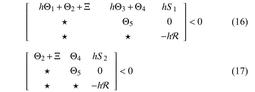
ford˙(t)∈{μ1,μ2} hold and where

with

Proof: The LKF is constructed as

where

Taking the time-derivative ofV(t) yields

where

then, we have

Applying Lemma 5 to κ (t) yields

where

and then by Lemma 6, it is obtained that

Hence, let ε (t)=?3(t), it is obtained that

wherea2=εT(t)Φ2ε(t) ,a1=εT(t)Φ1ε(t),a0=εT(t)Φ0ε(t)with

Furthermore, it is found thatf(d(t)) satisfies the quadratic function defined in (4) withz=d(t).Let

theinequalityV˙(t)<0 is satisfied based on Lemma 3 if the following conditions hold:

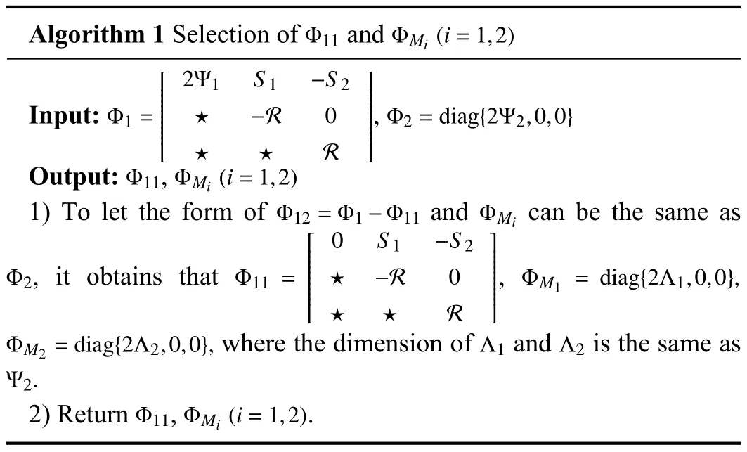
Algorithm 1 Selection of and Φ11 ΦMi(i=1,2)■■■■■■■■■■■■Φ2=diag{2Ψ2,0,0}Input: ,Φ11ΦMi(i=1,2)Φ1=■■■■■■■■■■■■Output: ,2Ψ1 S1 -S2? -R 0??R Φ2 Φ11 =ΦM2 =diag{2Λ2,0,0}, Λ1 Λ2 Ψ2 1) To let the form of and can be the same as, it obtains that ,where the dimension of and is the same as.Φ11ΦMi(i=1,2)Φ12=Φ1-Φ11 ΦMi■■■■■■■■■■■■0 S1 -S2? -R 0??R■■■■■■■■■■■■ ΦM1 = diag{2Λ1,0,0},2) Return ,.

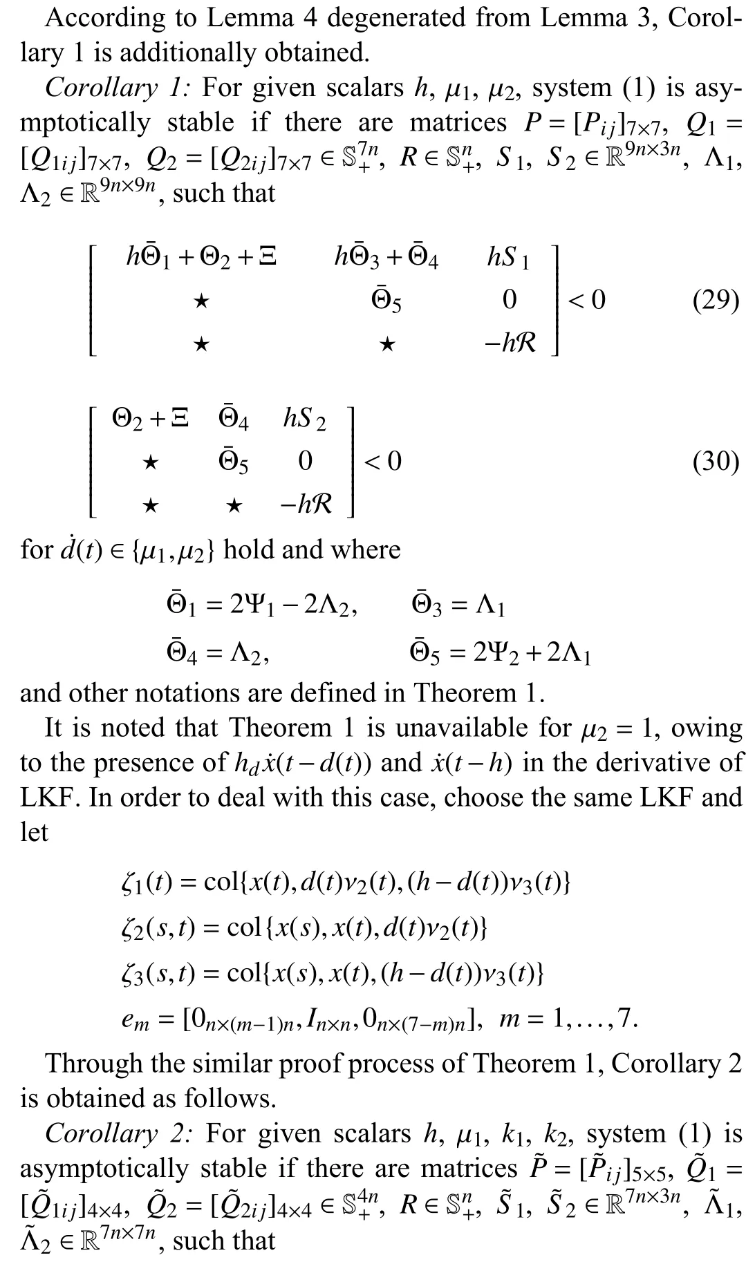
ford˙(t)∈{μ1,1} hold and where

with

and other notations are defined in Theorem 1.

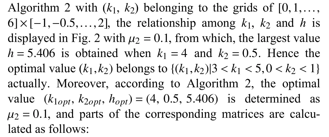
In Theorem 1, two adjustable parametersk1andk2are introduced, which are closely related to the determined MAUBhin this work.Hence, the range ofk1andk2is necessary to be adjusted to obtain the MAUBh.Furthermore, the following iterative optimization algorithm is designed, in which as one example,k10=1,k20=0 can be chosen initially.

Remark 6: The conservatism of results in Theorem 1 is reduced by the quadratic function convex approximation technique in Lemma 3 and ERCC in Lemma 6, compared to Lemmas 1 and 2.It also decreases the number of LMIs and simultaneously need not concern whethera2>0 ora2<0 actually,

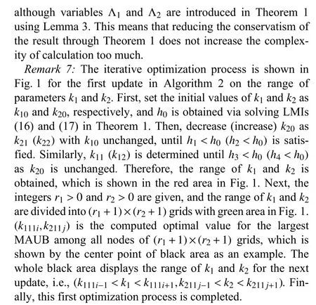
Algorithm 2 Obtain the Optimal Values of , and h.k1k2 Input: ),k1optk2opt hopt(k1,k2)=(k10,k20 h>0 Output: , and 1) Firstly calculate MAUB when ( ) = ( ), then let( ) = ( , ), ( ), ( ), ( , ), respectively, and the obtained MAUBs , , , are less than.Then we get an initial set , where ,, ,.l=1 l ≥p h0 k1,k2 k10,k20 k1,k2 k10 k21 k10,k22 k11,k20 k12 k20 h1h2h3h4 h0{(k1,k2)|k11100 k11li-k11li-1= k12l0-k11l0 3) Change set into new set, ,and are given integers.Let and.(i=1,2,...,r1) k21l j-k21lj-1= k22l0-k21l0 r1 r2 (j=1,2,...,r2)4) Check the LMI-based constrains in Theorem 1 by MATLAB,and calculate in case of belonging to a new set.Store and , where is the maximum of.k11l+10=k11li-1 k12l+10=k11li+1 k21l+10=k21li-1 k22l+10=hk1,k2 (k1,k2)hopt= hk11li,k21lj (k1opt,k2opt)=(k11li,k21lj) hk11li,k21lj hk1,k2 k215li)+1.Up date , , ,6) end k1opt, k2opt, hopt 7) Return.

V.NUMERICAL EXAMPLES

Three examples are provided in this section to verify the effectiveness and superiority of the developed theoretical results, and both the Yalmip toolbox of MATLAB R2015b and the SIMULINK are utilized for simulation.In the Examples 1-3, the number of iterationspfor all the numerical results is 2, and the grid node is (r1+1)×(r2+1)=7×7.

Example 1: Set system (1) with

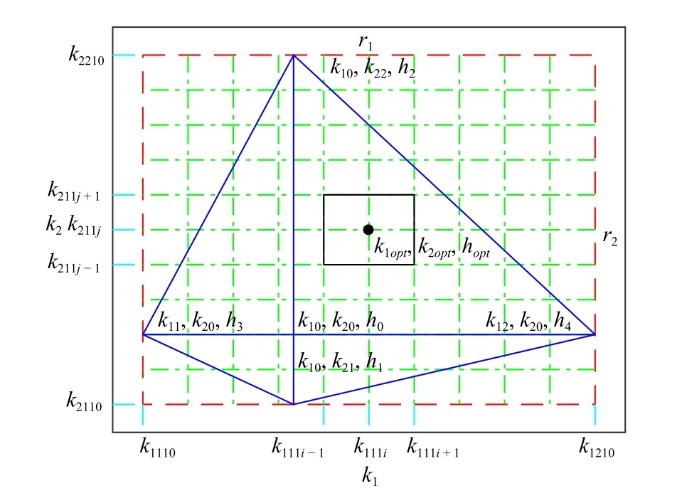
Fig.1.Iterative optimization process for optimal values of k1, k2, h at the first step.

which is always chosen as the general example about timedelay problems in the existing literatures.The MAUBs and the number of decision variables (NDVs) by Theorem 1 and Corollaries 1 and 2, and corresponding improvements over the best result (IBR) in the existing works can be seen at both Tables I and II as μ1=-μ2.And it can be concluded that although NDVs in Theorem 1 and Corollaries 1 and 2 are larger than others (except [21]), the MAUB is much larger than those in [2], [4]-[8], [16], [21], [24]-[28], [31], [32].Meanwhile, at Table I, when μ=0.1,0.5, the MAUBs obtained by Lemma 1 in [25], and Lemma 2 in [31] are(4.943, 3.317) and (4.958, 3.339), respectively, which are obviously less than (5.406, 3.733) of our work obtained by Lemma 3.Hence, it can be known that Lemma 3 is superior to Lemma 1 in [25], and Lemma 2 in [31].Besides, Table I shows the IBR with respect to MAUB is 7.2 % when μ2=0.1,5.4 % when μ2=0.5, respectively.And Table II displays that the improvement is 0.9 % as μ2=1.

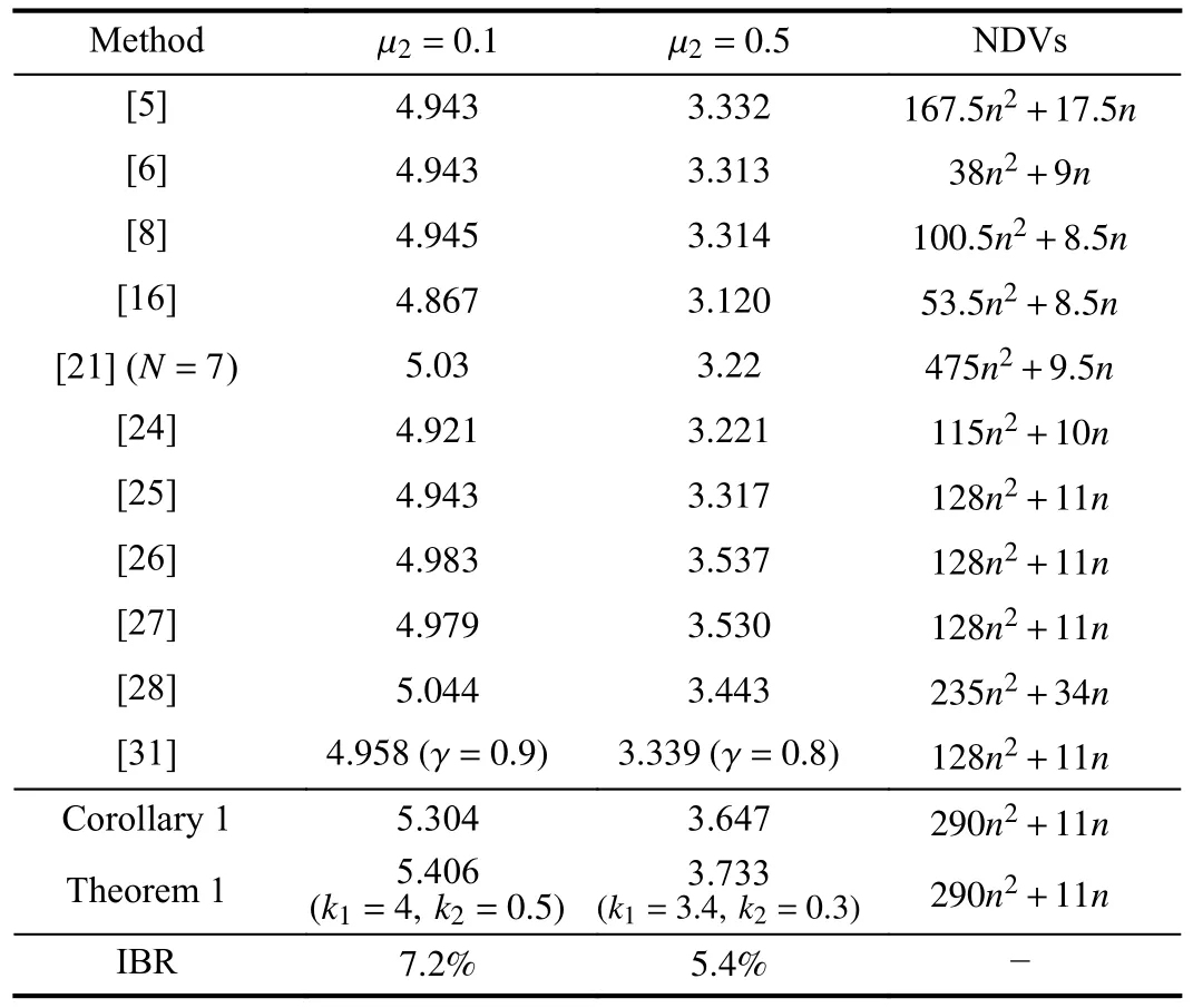
TABLE I THE MAUBS H FOR μ 1=-μ2 IN EXAMPLE 1

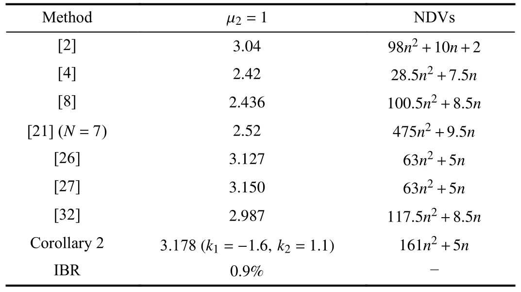
TABLE II THE MAUBS H FOR μ 1=-μ2 IN EXAMPLE 1

(k1opt,k2opt,hopt)=(3.4,0.3,3.733) as μ2=0.5 in similar steps.

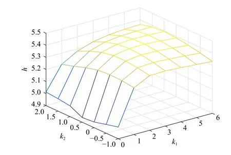
Fig.2.Relationship between h and two adjustable parameters k1, k2.

Set ? (t)=[2,2]T,t∈[-h,0], the state trajectories for system(1) with time-varying delays are shown in Fig.3 considering different types ofd(t) with sine wave and different values ofμ2.All the results demonstrate that the system is stable under different conditions, which fully verifies that our proposed approach is effective.

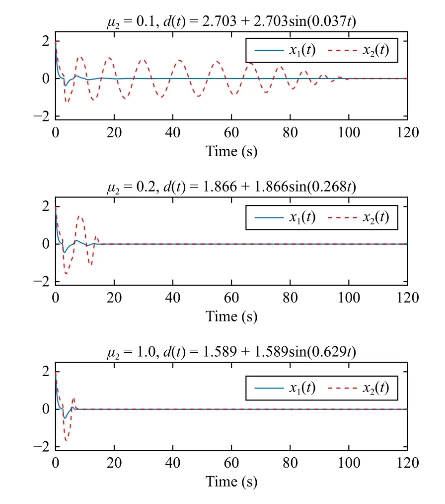
Fig.3.State responses in Example 1.

Example 2: For system (1) with

Both the MAUBs and their IBR by Theorem 1 and Corollary 1 are shown at Table III, from which it can be found that all MAUBs determined by our approach are larger than those obtained by other stability conditions in [5]-[8], [16], [21],[24], [26]-[29].For instance, the improvement with respect to MAUB is 48.2 % over the best result in [29] when μ2=0.1,and others can be seen at Table III.

Set ? (t)=[2,2]T,t∈[-h,0], and then the state responses are provided in Fig.4 when respectively considering different values ofd(t) in Fig.5.These results also verify the effectiveness of our developed method.

Example 3: Consider system (1) with

MAUBs for μ1=-μ2are shown at Table IV, from which it can be concluded that all MAUBs determined by Theorem 1 and Corollary 1 are larger than those via other stability conditions in [8], [16], [20], [21].It is worth noting that a stable region can be obtained only utilizing Theorem 1 and Corollary 1 as μ2becomes larger, e.g., μ2=0.2,0.5,0.8, while other existing results in [8], [16], [20], [21] can not get a feasible solution actually.This clearly shows Theorem 1 and Corollary 1 in our work outperforms the approaches in [8], [16],[20], [21].

Set ?(t)=[0.1,0.1]T,t∈[-h,0] withh=0.001, and then the state responses are provided in Fig.6 when respectively consideringd(t) with cosine wave and different values of μ2.These results also verify the effectiveness of our developedmethod.

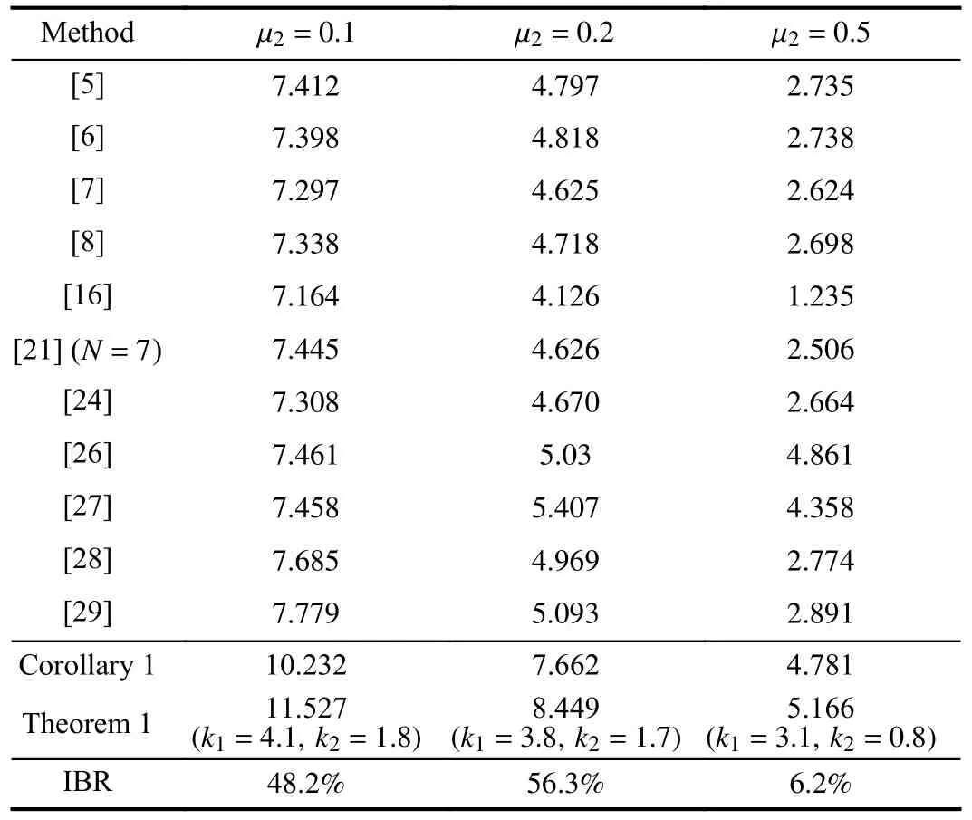
TABLE III THE MAUBS H FOR μ 1=-μ2 IN EXAMPLE 2

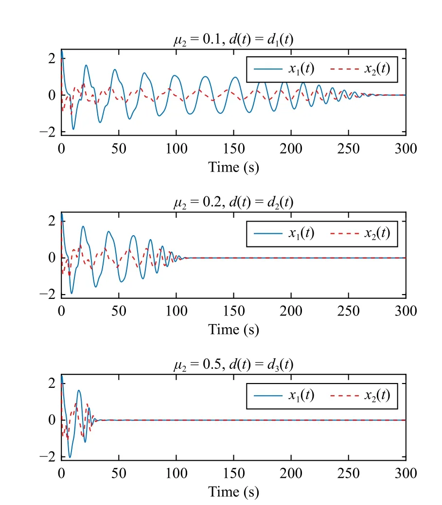
Fig.4.State responses in Example 2.

In summary, it can be seen from Tables I-IV that the results obtained by our work are less conservative than those obtained by references [2], [4]-[8], [16], [20], [21], [24]-[29],[31], [32] in Examples 1-3 through proposed Lemma 3 to estimate a tighter bound of the derivative of LKFs with the ERCC technique and the B-L inequality approach in our work.

VI.CONCLUSION

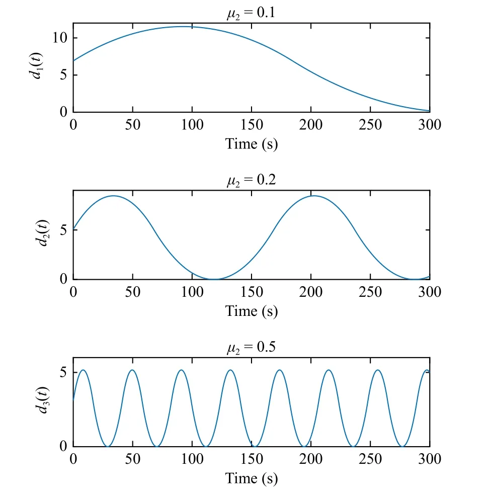
Fig.5.Time-delay d (t) with different derivatives in Example 2.

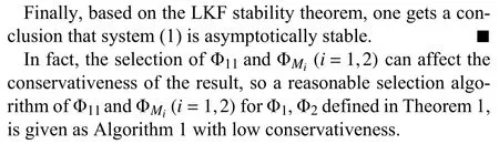
This paper develops a novel quadratic function convex approximation lemma and its application to the stability analysis for linear systems with time-varying delays.The quadratic function convex approximation technique is mainly to determine the negative definiteness of the quadratic functionf(z)deduced from the derivative of LKF.It is not necessary to consider the sign of the quadratic coefficienta2via introducing two adjustable parameters and two free variables.Based on the B-L inequality approach, the relaxed stability criteria for linear time-delay systems are established by using our developed lemma and the ERCC technique.The advantage and effectiveness of presented results are fully demonstrated via three numerical examples.

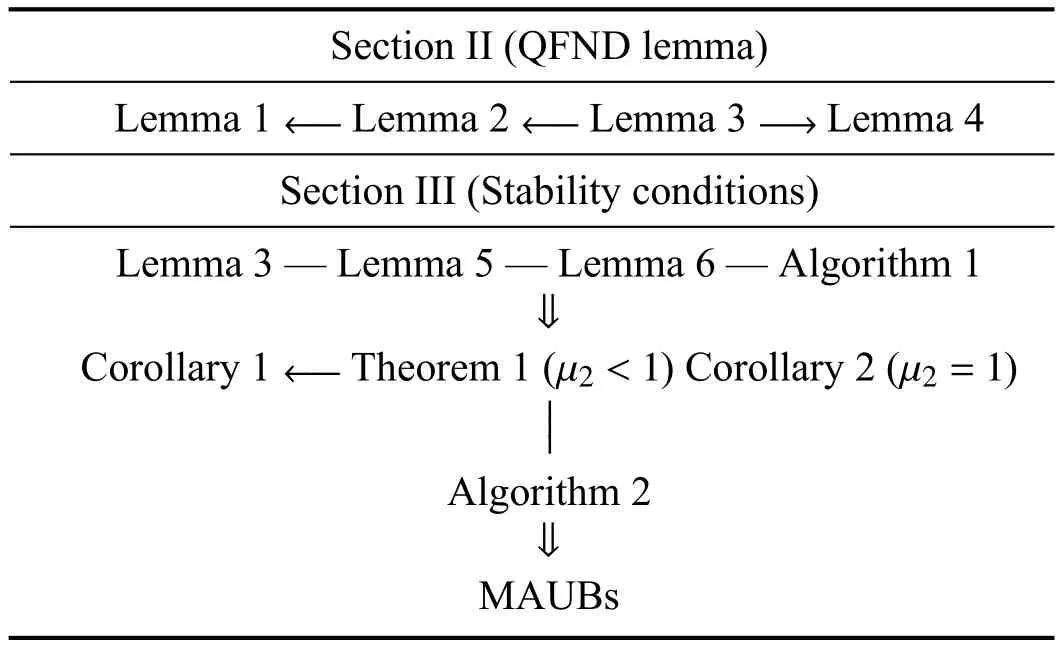
APPENDIX RELATION AMONG CONDITIONS

A solid arrow tells that a lemma, corollary or theorem can be degenerated into another (the pointed one), a solid line tells that lemmas, corollaries, theorems, or algorithms are combined on both sides,and a double arrow tells that a condition (the pointed one) can be derived from another.