Guancheng Wang | Zhihao Hao,2 | Haisheng Li | Bob Zhang,

1PAMI Research Group,Department of Computer and Information Science,University of Macau,Taipa,Macau, China

2China Industrial Control Systems Cyber Emergency Response Team, Beijing,China

3Beijing Key Laboratory of Big Data Technology for Food Safety, Beijing Technology and Business University,Beijing,China

Abstract This study proposes a novel gradient-based neural network model with an activated variable parameter, named as the activated variable parameter gradient-based neural network (AVPGNN) model, to solve time-varying constrained quadratic programming(TVCQP) problems.Compared with the existing models, the AVPGNN model has the following advantages: (1) avoids the matrix inverse, which can significantly reduce the computing complexity; (2) introduces the time-derivative of the time-varying parameters in the TVCQP problem by adding an activated variable parameter, enabling the AVPGNN model to achieve a predictive calculation that achieves zero residual error in theory; (3) adopts the activation function to accelerate the convergence rate.To solve the TVCQP problem with the AVPGNN model, the TVCQP problem is transformed into a non-linear equation with a non-linear compensation problem function based on the Karush Kuhn Tucker conditions.Then, a variable parameter with an activation function is employed to design the AVPGNN model.The accuracy and convergence rate of the AVPGNN model are rigorously analysed in theory.Furthermore, numerical experiments are also executed to demonstrate the effectiveness and superiority of the proposed model.Moreover, to explore the feasibility of the AVPGNN model, applications to the motion planning of a robotic manipulator and the portfolio selection of marketed securities are illustrated.

K E Y W O R D S computational intelligence, mathematics computing, optimisation

1 | INTRODUCTION

Quadratic programming (QP) problems are unique in many fields, including image processing [1], robotics [2] and the economy [3].In particular, a prevalent technology in object extraction named constrained energy minimisation can be classified as a static QP problem with equation constraints[1].In addition, compared with equality constraints, the inequality constraints extend the solution space, which can improve the detection accuracy [4].In portfolio selection,the variance of the portfolio is a time-varying QP problem that is subject to equations when the expected return is constant [3].Nowadays, with the rapid increase in data processing rates, many static QP problems have become time-varying, which require an online solving.Investigating the time-varying constrained QP (TVCQP) problem and designing effective solving methods for them have been a hot topic [5–7].

Typically, conventional numerical algorithms were originally designed for static problems, for example, the Newton iterative (NI) algorithm.They can also solve time-varying problems, while having poor accuracy due to the lack of velocity compensation for time-varying parameters.For instance,the steady-state residual error of the NI algorithm converges to O(τ), whereτdenotes the sampling interval of time-varying parameters [8].To further decrease the steady state residual error,Wang et al.inserted an integration feedback control into the NI algorithm, making the steady state residual error converge toO(τ2), which relieved the requirement of a high sampling rate [9].Besides Newton-type algorithms, gradientbased algorithms are another prevalent type of method.The gradient-based algorithms usually define a non-negative scalarvalued error function and then search the zero along the negative gradient direction[10].Gradient-based algorithms are wildly exploited in machine learning[11,12],optimisation[13,14] and image inpainting [15].Compared with the NI algorithm, gradient-based algorithms, for example, the original gradient neural network (OGNN) model, avoid the inverse of a matrix,which significantly reduces its computing complexity[16].Because of that, gradient-based algorithms are more popular in large-scale problems [17–19].For instance, the stochastic gradient descent method and its varieties are the most commonly employed to solve large-scale optimisation compared with the stochastic Newton-type algorithms.However, when solving time-varying problems, gradient-based algorithms also face the lagging error problem as the NI algorithm [20].

Recently, a special type of recurrent neural network named zeroing neural network (ZNN) models have attracted increasing attention due to its superior performance in solving time-varying problems [21–23].Differing from the gradient-based algorithms, the ZNN models construct an error function whose theoretical value is zero.Therefore,finding the theoretical solution can be interpreted as searching the zero-point of an error function.According to this conception, the original ZNN (OZNN) model properly defined the time derivative of the error function, which can achieve zero residual error [24].Compared with the numerical algorithms, ZNN models estimate the solution based not only on the current state but also the time derivative of the time-varying parameters.In other words, ZNN models can predict the future state of the parameters that successfully eliminate the lagging error existing in the NI and gradientbased algorithms.Regarding the OZNN model, it has been reported that it requires infinite convergence time (CT) [25].To remedy this deficiency, activation functions are utilised to shorten the CT.For instance, Zhang et al.employed a nonlinear activation function to form a new ZNN model, which has a superior convergence rate than the OZNN model [26].Furthermore, two non-linear activation functions are presented, making the ZNN model converge in pre-defined time and achieve a robust performance [27].Besides activation functions, varying parameters are also utilised to improve the convergence rate.Xiao et al.designed an Arctan-Type varying-parameter ZNN model, where the parameter includes the exponential of time and the power of time [28].In addition, Gerontitis et al.proposed a novel ZNN model exploiting a time-varying parameter to accelerate the convergence rate.However, these parameters may become infinite over time, which is unsuitable in practical applications[29].Furthermore, a piece-wise parameter is designed to enable the ZNN model to have various convergence rates at different time periods, which also successfully reduces the CT[30].Though ZNN models outperform other traditional algorithms in solving time-varying problems, their solving procedure involves the inversion of a matrix.On the one hand, the inversion of a matrix causes heavy computing load.On the other hand, the time-varying matrix needs to be nonsingular at every moment, which limits their feasibility.

In summary, Newton-type algorithms and ZNN models require the inversion of a matrix, while gradient-based algorithms avoid this.However, gradient-based algorithms suffer from lagging errors in solving time-varying problems.Therefore, this work aims to design a gradient-based neural network (GNN) model that also employs the time-derivative of parameters and achieves zero residual error.Firstly, a variable parameter is proposed in the GNN model, which can adjust the update step of the solution based on the current state of the residual error and the time-derivative of the parameters in problems.Then, activation functions are utilised in the variable parameter to improve the convergence rate of the model.Thus, an activated variable parameter GNN (AVPGNN) model is construed in this study, which not only inherits the advantage of being inversion-free in the gradient-based algorithms, but also enjoys zero residual error and the accelerated convergence rate as ZNN models.Furthermore, to utilise the AVPGNN model to solve the TVCQP problem, a non-linear compensation function is added into the Karush Kuhn Tucker (KKT) conditions to transform the TVCQP problem into a non-linear equation as well as a zero-searching problem.The AVPGNN model can efficiently estimate the solution of the TVCQP problem with zero residual error, which is proved theoretically.Moreover,the convergence rate of the AVPGNN model with various activation functions is discussed.To verify the theoretical analyses, numerical simulations and applications are provided,whose results demonstrate the superiorities of the proposed model.

The rest of this study is structured as follows.Section 2 introduces the TVCQP problem and its existing schemes.Then, Section 3 proposes the AVPGNN model and provides theoretical discussions regarding the accuracy and convergence rate.Afterwards, Sections 4 and 5 illustrate the stimulative results, including one numerical example and two applications.Lastly, Section 6 concludes this study and discusses potential research in the future.Before ending this introductory section, the highlights of this study are summarised below.

? A variable parameter with an activation function is added in the OGNN model to construct the AVPGNN model.

? The AVPGNN model is superior in accuracy, convergence rate and computing complexity when solving the TVCQP problem.

? The effectiveness and feasibility of the AVPGNN model have been verified by rigorous theoretical analyses and extensive experiments.

2 | PRELIMINARY THEORY

2.1 | Problem formulas

This study investigates the TVCQP problem expressed as follows:

where Equation (1) is the object function andTdenotes the transposition of a matrix or a vector.Meanwhile,y(t)∈Rndenotes the solution,A(t)∈Rn×nis a symmetric positive definite matrix, andb(t)∈Rn.Moreover, Equations (2) and(3) denote the equality and inequality constraints, whereC(t)∈Rl×nis a full-rank matrix,E(t)∈Rm×n,d(t)∈Rl,andf(t)∈Rm.Besides this, 0 denotes the vector or matrix that all elements equal to zero.To find out the optimal solutiony*(t), with two Lagrangian multiplier vectorsλ?1(t)∈Rlandλ?2(t)∈Rm, the TVCQP problem should satisfy the KKT conditions:

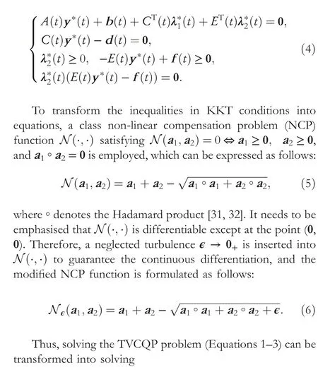
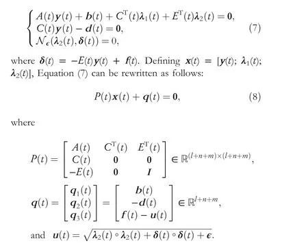
Besides this,Idenotes the identity matrix.Therefore, the TVCQP problem (Equations 1–3) has become the non-linear Equation (8).

2.2 | Existing schemes

2.2.1 | ZNN model

According to the framework of designing the ZNN model[33],an error function is constructed as follows:

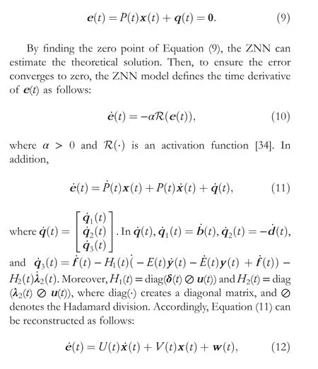
where

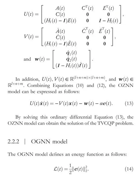
Starting with an initial point, the OGNN model finds the solution along with the negative gradient -?L(t)/?x(t) [35].According to Refs.[10, 36], the OGNN model solves the TVCQP problem as follows:

3 | THE PROPOSED AVPGNN MODEL

To obtain a higher accuracy,a variable parameter GNN model adopts a self-adaptive scalar parameter to adjust the step-size,which is formulated as follows:

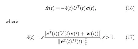
According to the definition ofV(t)andw(t),κcontains the time derivative of parameters in the TVCQP problem, indicating that the variable parameter GNN model can estimate the solution with zero residual error in theory just like the ZNN models.To demonstrate the global convergence of the proposed model, the following theorem is proven.

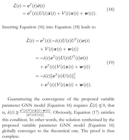
Theorem 1When solving the TVCQP problem with the proposed variable parameter GNN model(Equation 16),the computing solution can globally converge to the theoretical one.Proof: According to the Lyapunov stability theorem [37],L(t) is defined as a Lyapunov function.It is positive definite since L(t)>0 fore(t)≠0,and L(t)=0 if and only ife(t)=0.Then,according to Equation(12),the time derivative of L(t)is

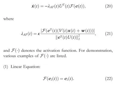
Regarding the ZNN models, they utilise various activation functions to accelerate the convergence rate.Therefore, activation functions are also considered for the variable parameter in Equation (16), and the AVPGNN model is designed as follows:

(2) Non-linear Equation 1:

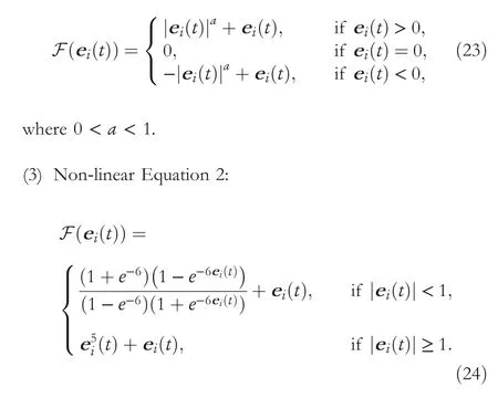
It should be noted that the variable parameter GNN model(Equation 16) is an AVPGNN model (Equation 20) activated by the linear Equation (22).Moreover, two non-linear activation functions(Equations 23 and 24)are provided to accelerate the convergence of the AVPGNN model (Equation 20).

Remark1 According to the proof in Theorem 1, the smaller ˙L(t) is, the faster the convergence rate the model has.The profiles of the activation functions (Equations 22–24) are shown in Figure 1, denoting that the outputs of non-linear activation functions (Equations 23 and 24) have larger absolute values than the linear Equation (22).In other words, the AVPGNN models activated by the non-linear equations have a faster convergence rate compared with the linear equation.Furthermore,since AVPGNN models(Equation 20)with nonlinear equations have smaller ˙L(t), they naturally satisfy the convergence condition in Theorem 1.

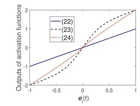
F I G U R E 1 The output profiles of various activation functions.

4 | NUMERICAL SIMULATIONS

In this section, the proposed AVPGNN model (Equation 20)is exploited to solve various TVCQP problems to demonstrate its effectiveness and feasibility.The experiments were performed in MATLAB 2019b on a desktop computer with a Core i7-7700 @3.60 GHz CPU, 16 GB memory and running Microsoft Windows 10.

4.1 | Numerical example

To verify the effectiveness of the proposed AVPGNN model(Equation 20), a numerical example of solving a TVCQP problem is provided.Consider a TVCQP problem expressed as follows:

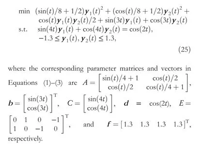
In this part, the OGNN (Equation 15) model and the AVPGNN (Equation 20) model activated by the linear Equation (22) are exploited to solve the TVCQP problem(Equation 25), whereβ= 10 andκ= 10.Their simulative results are demonstrated in Figures 2 and 3, respectively.The simulations started with five random initial states.The bluedotted curves in Figures 2a,b and 3a,b illustrate the computing solutionsy1(t) andy2(t), respectively.Meanwhile,the boundaries of solutions (-1.3 ≤y1(t),y2(t) ≤1.3) are denoted by the red curves.Compared with Figures 2 and 3,the computing solutions have obvious differences, especially at 1.8 and 4.8 s.The computing solutions of the AVPGNN model (Equation 20) at these moments are limited by inequalities, while those of the OGNN model (Equation 15) do not reach the boundary.Moreover, Figure 2c demonstrates the profile of the residual error of the OGNN model(Equation 15), which becomes steady at about 2 s.In addition, the maximum steady-state residual error (MSSRE) is 0.65, which is estimated by routine max in MATLAB among‖e(t)‖2after 2 s.According to Figure 3a,b, the computing solutions estimated by the AVPGNN model (Equation 20)not only converge to a certain solution, but also satisfy the constraints.In addition, Figure 3c shows its residual error ‖e(t)‖2, revealing that the AVPGNN model (Equation 20)converged within 1 s, and its MSSRE can reach the level of 10-4.Such small residual errors verify the effectiveness of the proposed AVPGNN model (Equation 20).

4.2 | Convergence rates

The convergence rates of the AVPGNN models activated by various activation functions are investigated in this part.Figure 4a depicts the residual error profiles withκ= 10,where the blue-solid curve, red-dotted curve and blackdashed curve denote the profiles of the activation functions(Equations 22, 23 and 24, respectively).The linear Equation (22) achieves the longest CT, that is, 0.80 s, while Equations (23) and (24) have shorter CTs, that is, 0.23 and 0.34 s, respectively.Moreover, according to the proof of Theorem 1, a largerκalso leads to a faster convergence rate.Figure 4b illustrates the residual error withκ= 50, where the CTs among various activation functions are much smaller than those ofκ= 10.Specifically, the CTs of Equations (22),(23), and (24) are 0.20, 0.14, and 0.15 s, correspondingly.In summary, utilising non-linear activation equations and enlargingκcan availably accelerate the convergence rate of the AVPGNN model (Equation 20).

F I G U R E 2 Simulative results of solving the TVCQP problem (Equation 25)by the OGNN model (Equation 16) from five random initial states.(a)The computing trajectories of y1(t)(blue-dotted line) versus their boundaries (red-solid line).(b) The computing trajectories of y2(t)(blue-dotted line) versus their boundaries (red-solid line).(c) The profiles of residual errors.

F I G U R E 3 Simulative results of solving the TVCQP problem(Equation 25)by the AVPGNN model(Equation 20)activated by the linear Equation (22)from five random initial states.(a)The computing trajectories of y1(t)(blue-dotted line)versus their boundaries(red-solid line).(b)The computing trajectories of y2(t) (blue-dotted line) versus their boundaries (red-solid line).(c) The profiles of residual errors.

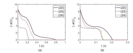
F I G U R E 4 Simulative results of solving the TVCQP problem (Equation 25) by the AVPGNN model (Equation 20) with various activation functions.(a) The results with κ = 10.(b) The results with κ = 50.

4.3 | Comparisons

To distinguish the superiority of the AVPGNN model (Equation 20),the comparison among various models(including the OGNN model [Equation 15], various ZNN models and the AVPGNN models [Equation 20]with various activation functions)are summarised in Table 1,whereβ=10 in Equation(15),α=10 for ZNN models,andκ=10 in Equation(20).Regarding the theoretical residual error, these models can obtain a zero residual error except for the OGNN model(Equation 15).Such a difference in theoretical residual error is reflected in that the OGNN model (Equation 15) has a much larger MSSRE(7.0×10-1)when solving the TVCQP problem.The MSSREs of other models are near zero numerically, which is not consistent with the theoretical zero residual error.This is due to the finite accuracy of the digital computer executing algorithms.Moreover, AVPGNN(Equation 20) models are inversion-free of matrices, releasing the constraints of time-varying parameters of TVCQP problems and reducing the computing complexity.Furthermore,regarding the CT,the OGNN model(Equation 15)achieves a shorter CT than the AVPGNN model(Equation 16) activated by the linear Equation (22), while the OGNN (Equation 15) model has a much larger RMMSE.Accelerated by the activation functions(Equations 23 and 24),the AVPGNN model (Equation 20) produces a much shorter CT (0.23 and 0.34 s), demonstrating the effectiveness of the non-linear activation function.Furthermore,compared with the ZNN models activated by non-linear activation functions in Refs.[20, 23], the AVPGNN models with Equations (23) and(24)obtain shorter CTs and smaller MSSREs.

5 | APPLICATIONS

5.1 | Robot motion planning

In this part,the AVPGNN model(Equation 20)is exploited in controlling the robotic manipulator to draw the Rhodonea curve, where the task can be modelled as follows:

whereθ(t) andr(t) denote the joint-angle and end-effector position, respectively.Correspondingly, ˙θ(t) is the joint velocity, while ˙r(t) is the end-effector velocity [38].In realistic kinematic control,the manipulator is physically limited in joint velocity, whose lower and upper boundaries are ˙θ-(t) and ˙θ+(t), correspondingly [39].The simulation started from the initial stateθ(0)=[0π/4 0π/2-π/4 0]Twith ˙θ-(t)=-0.5 rad/s and ˙θ+(t)=0.5 rad/s, and the simulation time for this task is 10 s.In addition,the AVPGNN model(Equation 20)is activated by the linear Equation (22), andκ= 102.

The experimental results are shown in Figure 5.Figure 5a depicts the actual trajectories of the whole robotic manipulator,where the end-effector successfully generated a Rhodonea curve.To evaluate the accuracy of the AVPGNN model(Equation 20), the comparison between the desired path and the actual path is demonstrated in Figure 5b.The actual path(red-dotted curve) can well follow the desired one (blue-solid curve).Moreover, Figure 5c shows the position errors in a three-dimensional space, where the position errors are at the level of 10-4m,indicating the high accuracy of the AVPGNN model (Equation 20).Furthermore, Figure 5d shows the profiles of ˙θin the TVCQP problem (Equation 26).All the elements of the computing solution are in the range [-0.5, 0.5]rad/s,which satisfy the inequality constraints in Equation(26).

5.2 | Portfolio selection

In this part, the proposed AVPGNN model (Equation 20) is employed in portfolio selection, which aims to achieve higher profits.In recent years, the time-varying portfolio selection problem has been deemed an effective method to assess investments and find opportunities (deals) [3, 5].Assuming that there arekmarketed securities in a portfolio,and the space of portfolio is denoted asj(t) = [j1(t),j2(t), …,jk(t)], whereji(t),i= 1, …,kdenotes the price of theith security.hiis the expected return estimated by the simple moving average

T A B L E 1 Comparison among various models for solving the TVCQP problem (Equation 25).

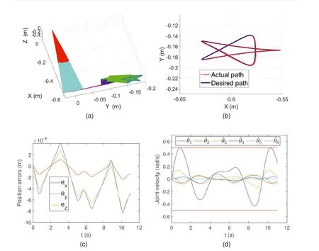
F I G U R E 5 Experimental results of robotic manipulator motion planning synthesised by the AVPGNN model(Equation 20)solving the TVCQP problem(Equation 26).(a)The synthesising trajectories of the robotic manipulator in the Cartesian space.(b)The computing trajectories(red-dotted curve)versus the desired path (blue-solid curve).(c) Profiles of position errors of the end-effector.(d) Profiles of joint velocities and their inequality constraints.

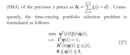
whereη(t) is the portfolio.In addition,Q(t) denotes the covariance matrix ofj(t) andre(t) denotes the target expected return of the portfolio.

In this simulation, four securities are investigated, whose financial time series are real-world data taken from https://finance.yahoo.com/.j(t) includes the data from 2 April 2019 to 1 September 2019, while the span ofh(t) is from 1 May 2019 to 1 September 2019.Moreover, the discrete-time series are linearly interpolated to form the TVCQP problem(Equation 27) as Ref.[5].The time periodτof SMA is set as 20, andre(t) = 0.962.Furthermore,κ= 2 × 104in the AVPGNN model (Equation 20).The simulative results are plotted in Figure 6, where Figure 6a demonstrates the portfolio, and Figure 6b shows the expected return of the portfolio.In Figure 6a, the computing solution is in the range [0,1], satisfying the constraints 0 ≤η(t) ≤1.According to Figure 6b, with such a portfolio, the return (purple curve) is larger thanre(t) (red-dotted curve) after the middle of May.Moreover, SMA20 (black curve) denotes the mean return of the market, which is lower than the return generated by the AVPGNN model (Equation 20).In other words, solving the portfolio selection problem by the AVPGNN model (Equation 20) can achieve more profits than holding each security on average.

F I G U R E 6 Simulative results of solving the portfolio selection problem (Equation 27) by the AVPGNN model (Equation 20).(a) The trajectories of portfolio η(t).(b) The trajectories of expected return.

6 | CONCLUSION

This article presented an AVPGNN model utilising an activated variable parameter to solve the TVCQP problem.The AVPGNN model not only inherits free of the inverse of a matrix in the OGNN model, but also achieves zero residual error and adopts activation function like ZNN models.The theoretical analyses indicate that the AVPGNN model can globally converge to the theoretical solution.and the nonlinear activation function can accelerate the convergence rate.In addition, extensive experiments are performed.Numerical experimental results verify the correctness of the theoretical analyses and illustrate the superiority of the AVPGNN model compared with other models.Furthermore, the AVPGNN model is successfully employed to control the manipulator conducting the Rhodonea curve and manage a portfolio to achieve the additional profit, demonstrating the remarkable potential in various applications.

In the future, other superior properties of the AVPGNN model should be pursued and investigated, enabling its application in other real-world applications.For example, the integration of historical residual errors can be inserted into the proposed model to achieve noise suppression.Moreover, the finite-time convergence AVPGNN model based on elaborately designed activation functions should be investigated in the future.

ACKNOWLEDGEMENTS

This work was supported in part by the University of Macau(File No.MYRG2018-00053-FST), in part by the Open Research Fund of the Beijing Key Laboratory of Big Data Technology for Food Safety (Project No.BTBD-2021KF05),in part by the Major Science and Technology Special Project of Yunnan Province (202102AD080006).

CONFLICT OF INTEREST STATEMENT

The author declares that there is no conflict of interest that could be perceived as prejudicing the impartiality of the research reported.

DATA AVAILABILITY STATEMENT

Data sharing is not applicable to this article as no data sets were generated or analysed during the current study.

ORCID

Bob Zhanghttps://orcid.org/0000-0003-2497-9519