Nguyen Xuan LINH

Department of Mathematics Mathematics, Falcuty of Information Technology,National University of Civil Engineering E-mail: linhnx@nuce.edu.vn

Duong Viet THONG?

Division of Applied Mathematics, Thu Dau Mot University, Binh Duong Province, Vietnam E-mail: duongvietthong@tdmu.edu.vn

Prasit CHOLAMJIAK

School of Science, University of Phayao, Phayao 56000, Thailand E-mail: prasitch2008@yahoo.com

Pham Anh TUAN Luong Van LONG

Faculty of Mathematical Economics, National Economics University, Hanoi City, Vietnam E-mail: patuan.1963@gmail.com; longtkt@gmail.com

Abstract In this work,we investigate a classical pseudomonotone and Lipschitz continuous variational inequality in the setting of Hilbert space, and present a projection-type approximation method for solving this problem. Our method requires only to compute one projection onto the feasible set per iteration and without any linesearch procedure or additional projections as well as does not need to the prior knowledge of the Lipschitz constant and the sequentially weakly continuity of the variational inequality mapping. A strong convergence is established for the proposed method to a solution of a variational inequality problem under certain mild assumptions. Finally, we give some numerical experiments illustrating the performance of the proposed method for variational inequality problems.

Key words Inertial method; Tseng’s extragradient; viscosity method; variational inequality problem; pseudomonotone mapping; strong convergence

1 Introduction

Let H be a real Hilbert space with the inner product 〈·,·〉 and the induced norm ‖·‖. Let C be a nonempty closed convex subset in H.

The purpose of this paper is to consider the classical variational inequality problem (VI)[12, 13], which is to find a point x?∈C such that

where F : H →H is a mapping. The solution set of (1.1) is denoted by Sol(C,F). In this paper, we assume that the following conditions hold:

Condition 1.1 The solution set Sol(C,F) is nonempty.

Condition 1.2 The mapping F :H →H is pseudomonotone, that is,

Condition 1.3 The mapping F :H →H is L-Lipschitz continuous, that is, there exists L>0 such that

Recently, many numerical methods have been proposed for solving variational inequalities and related optimization problems; see [4-7, 17-19, 23, 29, 41].

One of the most popular methods for solving the problem(VI)is the extragradient method(EGM) which was introduced in 1976 by Korpelevich [20] as follows:

where F : H →H is monotone and L-Lipschitz continuous on C, λ ∈(0,1L) and PCdenotes the metric projection from H onto C.

In recent years, there are many results which had been obtained by the extragradient method and its modifications when F is monotone and L-Lipschitz continuous in infinitedimensional Hilbert spaces (see, for instance, [2, 8, 21, 24, 28, 36, 38, 39]).

In [4], Censor et al. introduced the subgradient extragradient method (SEGM), in which the second projection onto C is replaced by a projection onto a specific constructible half-space:

where Tn={w ∈H :〈xn-λFxn-yn,w-yn〉≤0}, F :H →H is monotone and L-Lipschitz continuous on H, λ ∈(0,1L). Under several suitable conditions, it is shown in [4] that any sequence {xn} generated by the subgradient extragradient method (SEGM) converges weakly to an element of Sol(C,F).

Since in infinite dimensional spaces norm convergence is often more desirable, a natural question which raises is: How to design and modify the extragradient method (EGM), the subgradient extragradient method (SEGM) and related results such that strong convergence is obtained?

In order to answer to the above question, in[27], Nadezhkina and Takahashi introduced an iterative process for solving Sol(C,F) (1.1) when F is a monotone and L-Lipschitz-continuous mapping using the two well-known hybrid method and extragradient method:

Algorithm 1.4

where Cn={z ∈C :‖zn-z‖≤‖xn-z‖},Qn={z ∈C :〈xn-z,x1-xn〉≥0},F :H →H is monotone on C and L-Lipschitz continuous on C,λ ∈(0,1L). This iterative process(1.2),which consists of two projections onto the feasible set C and another projection onto the intersection of half-spaces Cnand Qnper iteration, seems difficult to use in practice when C is a general closed and convex set.

In[5], Censor et al. also introduced the following hybrid subgradient extragradient method(HSEGM) to obtain strong convergence result for Sol(C,F) (1.1) with a monotone and LLipschitz-continuous mapping F using this method: x1∈H:

Algorithm 1.5

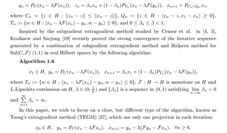
where F :H →H is monotone and L-Lipschitz continuous on H, λ ∈(0,1L).

The purpose of this work is to investigate the strong convergence theorem for solving pseudomonotone variational inequalities in real Hilbert spaces. The proposed algorithm is a combination between the inertial Tseng extragradient method [34] and the viscosity method[25] with the technique of choosing a new step size. The advantage of the algorithm is the computation of only two values of the inequality mapping and one projection onto the feasible set per iteration, and the strong convergence is proved without the prior knowledge of the Lipschitz constant as well as does not need to requires the sequentially weakly continuity of the variational inequality mapping, which distinguishes our method from projection-type method for variational inequality problems with monotone mappings which was recently studied in[35].Finally, we give some numerical experiments for the performance of the proposed algorithm for variational inequality problems.

This paper is organized as follows: in Section 2, we recall some definitions and preliminary results for further use. Section 3 deals with analyzing the convergence of the proposed algorithm.Finally, in Section 4, we perform some numerical experiments to illustrate the behaviours of the proposed algorithm in comparison with other algorithms.

2 Preliminaries

Let H be a real Hilbert space and C be a nonempty closed convex subset of H.? The weak convergence of {xn} to x is denoted by xn?x as n →∞;

? The strong convergence of {xn} to x is written as xn→x as n →∞.

For each x,y ∈H, we have the following:

11. Gold: Gold, as always, is a precious metal and was reserved for the wealthy in past centuries. Gold has often been used for money and jewelry, to represent wealth and power.

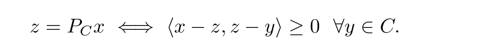
For all point x ∈H, there exists the unique nearest point in C, denoted by PCx, such that

PCis called the metric projection of H onto C. It is known that PCis nonexpansive.

Lemma 2.1 ([14]) Let C be a nonempty closed convex subset of a real Hilbert space H.For any x ∈H and z ∈C, we have

For some more properties of the metric projection, refer to Section 3 in [14].Definition 2.2 Let F :H →H be a mapping. F is called monotone if

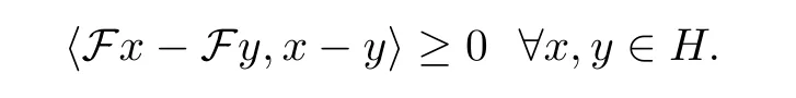
It is easy to see that every monotone operator F is pseudomonotone, but the converse is not true; see [18].

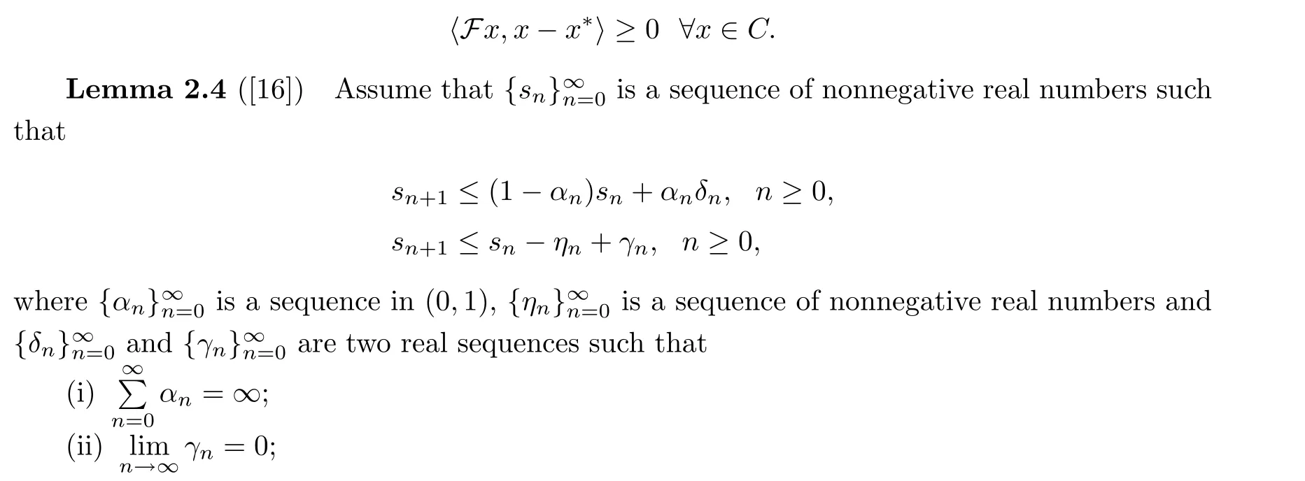
Lemma 2.3 ([5,Lemma 2.1]) Consider the problem Sol(C,F)with C being a nonempty,closed, convex subset of a real Hilbert space H and F : C →H being pseudo-monotone and continuous. Then, x?is a solution of Sol(C,F) if and only if

3 Main Results

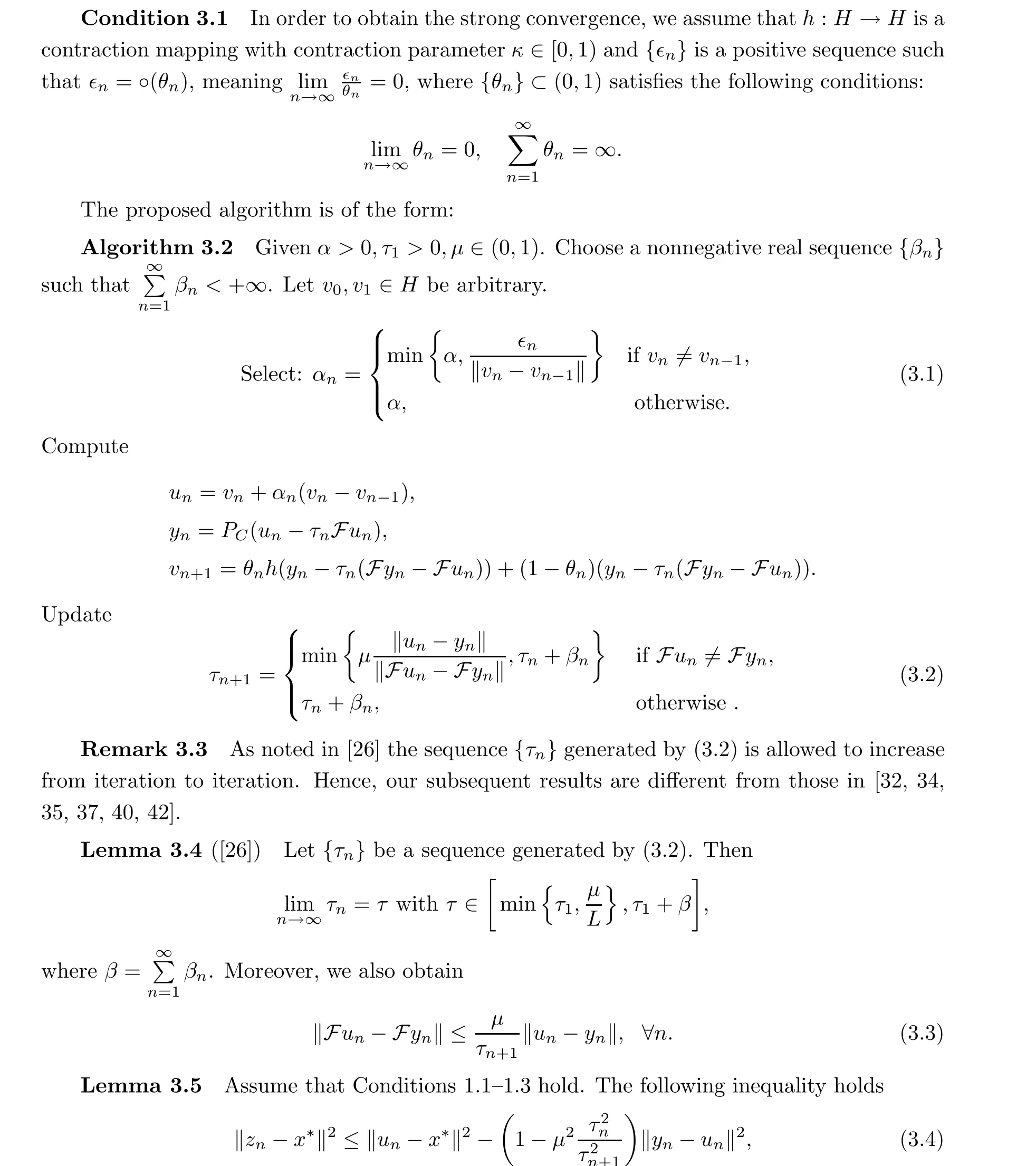
where zn:=yn-τn(Fyn-Fun).

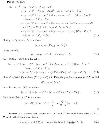
then the sequence {vn} generated by Algorithm 3.2 converges strongly to an element x?∈Sol(C,F), where x?=PSol(C,F)?h(x?).

Remark 3.7 It is obviously that if F is sequentially weakly continuous, then F satisfies condition (3.9) but the inverse is not true. This is the assumption which has frequently been used in recent articles on pseudomonotone variaional inequality problems, for example, [9, 30,32, 38, 43]. Moreover,when F is monotone, we can remove condition (3.9) (see [11, 38]).

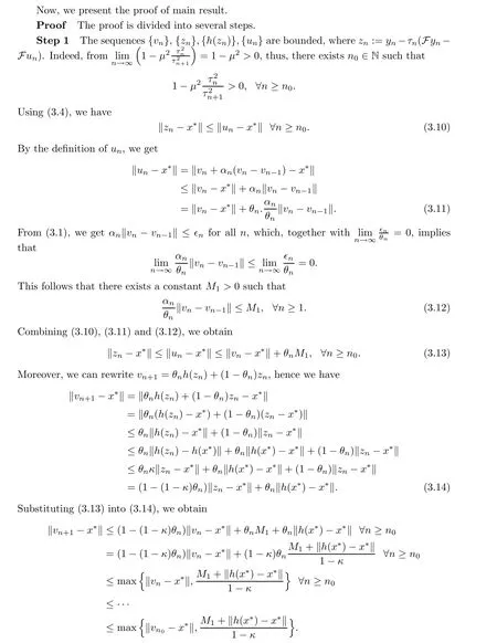
This implies that {vn} is bounded. We also get that {zn},{h(zn)}, and {un} are bounded.

Remark 3.8 Our result generalizes some related results in the literature and hence might be applied to a wider class of nonlinear mappings. For example,in the next section,we presented the advantages of our method compared with the recent results [5, Theorem 3.2], [5, Theorem 3.1] and [5, Theorem 3.1] as follows:

(i) In Theorem 3.6, we replaced the monotonicity by the pseudomonotonicity of F.

(ii) The fixed stepsize is replaced by the adaptive stepsizes according to per iteration, and this modification, which follows the proposed algorithm, is proved without the prior knowledge of the Lipschitz constant of mapping.

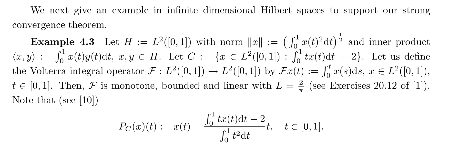
4 Numerical Illustrations

We next provide some numerical experiments to validate our obtained results in some Hilbert spaces.

Example 4.1 This first example (also considered in [22, 24]) is a classical example for which the usual gradient method does not converge. It is related to the unconstrained case of Sol(C,F) (1.1), where the feasible set is C := Rm(for some positive even integer m) and F :=(aij)1≤i,j≤mis the square matrix m×m whose terms are given by

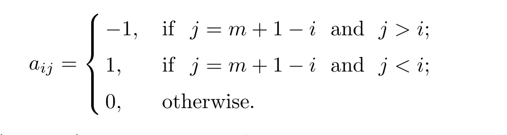
The zero vector z = (0,··· ,0) is the solution of this test example. To compare Algorithm 1.6 and Algorithm 3.2, we take θn= 1/1000(n+1), α = 0.5, εn= 1/n2, τ1= 0.3, λn= 0.15/L andμn=0.5 for all n ≥1. Let v0and v1be initial points whose elements are randomly chosen in the closed interval [-1,1]. We terminate the iterations if ‖F(xiàn)vn‖2≤ε with ε = 10-5. The results are listed on Table 1.

Table 1 Comparison of Algorithm 1.4, Algorithm 1.5, Algorithm 1.6 and Algorithm 3.2 for Example 4.1

Example 4.2 This example is taken from[15] and has been considered by many authors for numerical experiments (see, for example, [23, 31]). The operator F is defined by Fx =Mx+q, where M = BTB+S+D, and S,D ∈Rm×mare randomly generated matrices such that S is skew-symmetric(hence the operator does not arise from an optimization problem),D is a positive definite diagonal matrix(hence the variational inequality has a unique solution)and q =0. The feasible set C is described by linear inequality constraints Bx ≤b for some random matrix B ∈Rm×kand a random vector b ∈Rkwith nonnegative entries. Hence the zero vector is feasible and therefore the unique solution of the corresponding variational inequality. These projections are computed by solving a quadratic optimization problem using the MATLAB solver quadprog. Hence,for this class of problems,the evaluation of F is relatively inexpensive,whereas projections are costly. We present the corresponding numerical results (number of iterations and CPU times in seconds) using different dimensions m and numbers of inequality constraints k. In this example, we choose θn= 1/500(n+5), α = 0.5, εn= 1/n2, τ1= 0.001,λn= 0.1/L, μn= 0.01 for all n ≥1 and h(x) = x/2. Let v0and v1be initial points whose elements are randomly chosen in the closed interval [0,1]. We terminate the iterations if‖vn-PC(vn-Fvn)‖2≤ε with ε=10-5. The results are shown on Table 2.

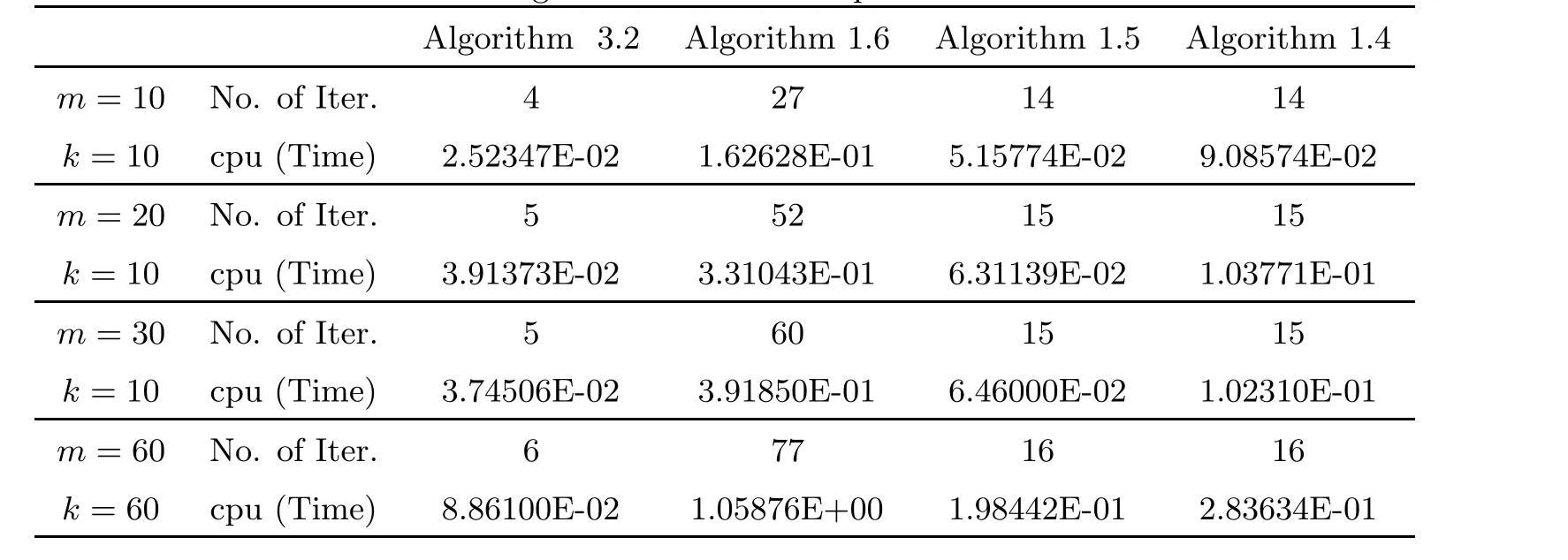
Table 2 Comparison of Algorithm 1.4, Algorithm 1.5, Algorithm 1.6 and Algorithm 3.2 for Example 4.2

In Example 4.3, we take f(x) = x/15, θn= 1/(130n+5), α = 0.5, εn= 1/n1.1, τ1= 0.002,λn=π/27 and μn=0.001 for all n ≥1. We terminate the iterations if En=‖vn+1-vn‖≤ε with ε = 10-5. The numerical results are listed on Table 3. Furthermore, we illustrate the convergence behavior of the sequences generated by all algorithms in Figures 1-4.

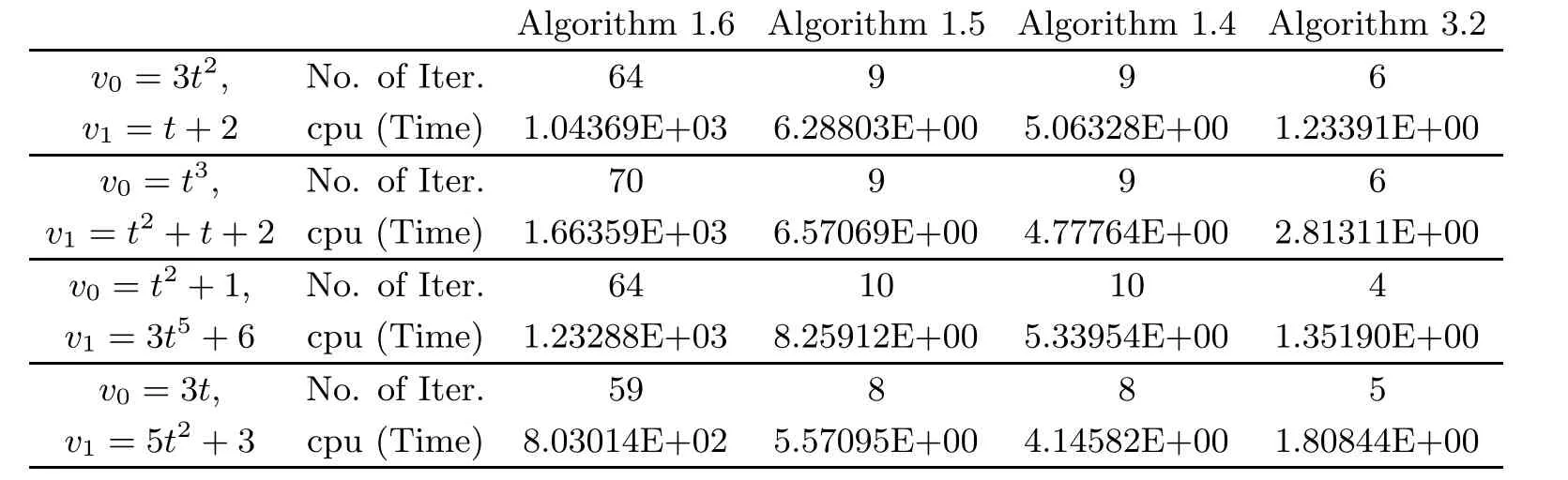
Table 3 Comparison of Algorithm 1.4, Algorithm 1.5, Algorithm 1.6 and Algorithm 3.2 for Example 4.3

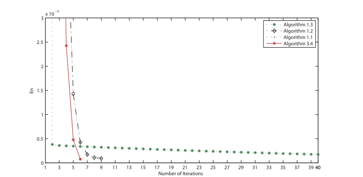
Figure 1 Comparison of four algorithms in Example 4.3 when v0 =3t2 and v1 =t+2

Figure 2 Comparison of four algorithms in Example 4.3 when v0 =t3 and v1 =t2+t+2

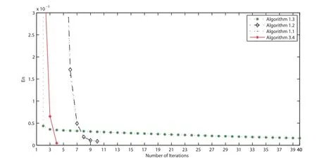
Figure 3 Comparison of four algorithms in Example 4.3 when v0 =t2+1 and v1 =3t5+6

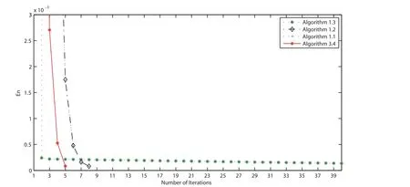
Figure 4 Comparison of four algorithms in Example 4.3 when v0 =3t and v1 =5t2+3

Finally, we discuss the strong convergence of the proposed Algorithm 3.2 in case α = 0.5(hence αn/= 0) and αn= 0 (without inertial term). The numerical results are reported in Table 4, and we take f(x) = x/15, θn= 1/(200n+5), εn= 1/n1.1, τ1= 0.2 and μn= 0.7 for all n ≥1. The comparisons are demonstrated in Figures 5-8.

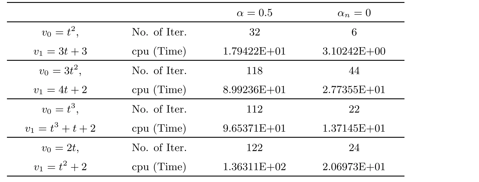
Table 4 Comparison of Algorithm 3.2 for Example 4.3 with α=0.5 and αn =0

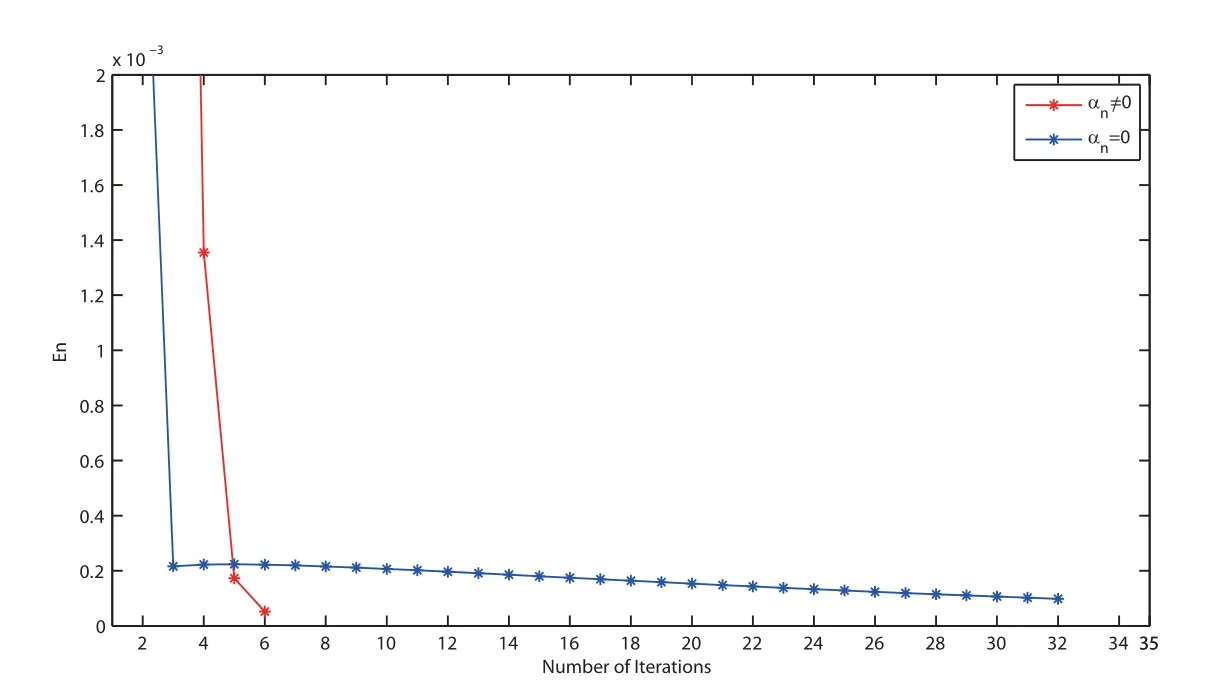
Figure 5 Comparison of Algorithm 3.2 for Example 4.3 when v0 =t2 and v1 =3t+3

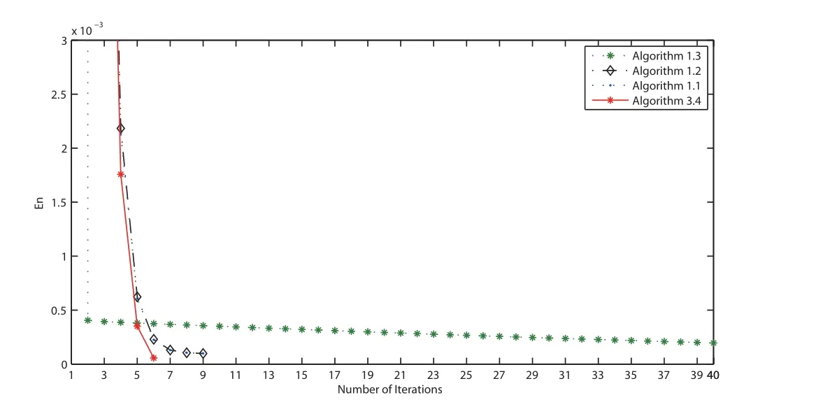
Figure 6 Comparison of Algorithm 3.2 for Example 4.3 when v0 =3t2 and v1 =4t+2

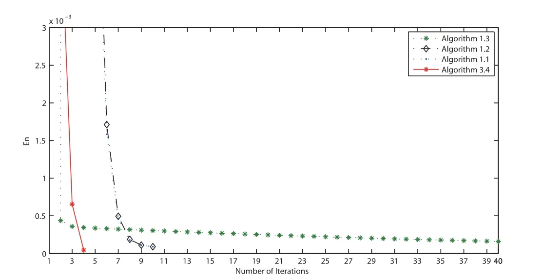
Figure 7 Comparison of Algorithm 3.2 for Example 4.3 when v0 =t3 and v1 =t3+t+2

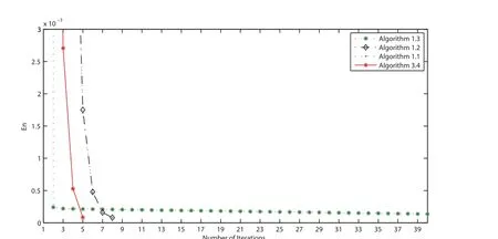
Figure 8 Comparison of Algorithm 3.2 for Example 4.3 when v0 =2t and v1 =t2+2

5 Conclusions

The paper has proposed a new method for solving pseudomonotone and Lipschitz VIs in Hilbert spaces. Under some suitable conditions imposed on parameters, we prove the strong convergence of the algorithm. The efficiency of the proposed algorithm has also been illustrated by several numerical experiments.