Muyassar Ahmat and Jianxian Qiu

School of Mathematical Sciences and Fujian Provincial Key Laboratory of Mathematical Modeling and High-Performance Scientific Computing,Xiamen University,Xiamen 361005,China.

Abstract.In this article,we present a third-order weighted essentially non-oscillatory(WENO)method for generalized Rosenau-KdV-RLW equation.The third order finite difference WENO reconstruction and central finite differences are applied to discrete advection terms and other terms,respectively,in spatial discretization.In order to achieve the third order accuracy both in space and time,four stage third-order L-stable SSP Implicit-Explicit Runge-Kutta method(Third-order SSP EXRK method and thirdorder DIRK method)is applied to temporal discretization.The high order accuracy and essentially non-oscillatory property of finite difference WENO reconstruction are shown for solitary wave and shock wave for Rosenau-KdV and Rosenau-KdV-RLW equations.The efficiency,reliability and excellent SSP property of the numerical scheme are demonstrated by several numerical experiments with large CFL number.

Key words:Rosenau-KdV-RLW equation,WENO reconstruction, finite difference method,SSP implicit-explicit Runge-Kutta method.

1 Introduction

The nonlinear wave behavior is one of the active scientific research areas during the past several decades.Numerical solution of nonlinear wave equations is significantly necessary since most of these types of equations are not solvable analytically in the case of the nonlinear terms are included.

Many mathematical models,especially nonlinear partial differential equations describe various types of wave behavior in nature.Typically,the KdV equation(Kortewegde Vries equation)is suitable for small-amplitude long waves on the surface of the subject,such as shallow water waves,ion sound waves,and longitudinal astigmatic waves.RLW equation(Regularized Long-Wave equation)can describe not only shallow water waves,but also nonlinear dispersive waves,ion-acoustic plasma waves,magnetohydrodynamic plasma waves.The Rosenau equation[1]was proposed for explaining the dynamic of dense discrete systems since the case of wave-wave and wave-wall interactions can not be explained by the KdV and RLW equations.

In order to further consider the nonlinear wave behavior,the viscous termuxxxoruxxtneed to be included in Rosenau equation,which leads to the achievement of Rosenau-RLW equation:

or Rosenau-KdV equation:

There have been many difficulties in evaluating analytical solutions of nonlinear dispersive wave equations and so on the development of numerical schemes.Even so,one derived the solitary wave solution and singular soliton solution for the Rosenau-KdV equation by the ansatz method as well as the semi-inverse variational principle[2]while the shock wave solution of this equation was determined for two particular values of the power law nonlinearity parameterp=3 andp=5 by Ebadi[3].

Significant numerical studies have been done on the Rosenau-KdV equation[4,5].Two-level nonlinear implicit Crank-Nicolson difference scheme and three-level linearimplicit difference scheme were presented to solve two-dimensional generalized Rosenau-KdV equation by Atouani[4].Their experiment proved that both schemes were uniquely solvable,unconditionally stable and second-order convergent inL1norm,the linearized scheme was more effective in terms of accuracy and computational cost.Wang and Dai[5]proposed a conservative unconditionally stable finite difference scheme withO(h4+τ2)for the generalized Rosenau-KdV equation in both one and two dimension,wherehis spatial step andτis temporal step,respectively.

A mass-preserving scheme which combined a high-order compact scheme and a threelevel average difference iterative algorithm was analyzed and tested for the Rosenau-RLW equation in[6].In their work,they focused on the development of the approach for solving the nonlinear implicit scheme in aim to improve the accuracy of approximate solutions.The Rosenau-RLW equation was also solved by second-order nonlinear finite element Galerkin-Crank-Nicolson method which was linearized by predictor-correction extrapolation technique in[7].An energy conservative two-level fourth-order nonlinear implicit compact difference scheme for three dimensional Rosenau-RLW equation was designed by Li[8]and an iterative algorithm was introduced to generate this nonlinear algebraical system.

In this paper,we focus on one-dimensional generalized Rosenau-KdV-RLW equation.This model is difficult to solve numerically because of the excessive computational cost caused by high order mixed derivative term and the selective wave behavior caused by the power law nonlinearity term.In order to keep this model in a generalized setting,the Rosenau-KdV-RLW equation is written as:

whereu(x,t)denote the profile of the wave whilexandtare the spatial and temporal variables,respectively.α>0,ε>0 are the parameters of linear and nonlinear advection terms,p≥2 is the parameter of power law nonlinearity.θ,δ,νare the parameters of KdV,RLW,Rosenau terms,respectively.

Rosenau-KdV-RLW equation has been studied both theoretically and numerically in recent years.Ansatz approach and semi-inverse variational principle were used to determine the solitary and shock solution,and the conservation laws of the Rosenau-KdVRLW equation with power law nonlinearity were computed by the aid of multiplier approach in Lie symmetry analysis in[9]and[10].A three-level second-order accurate weighted average implicit finite difference scheme was presented by Wongsaijai[11]to solve the Rosenau-KdV-RLW equation.Wang[12]introduced a three-level linear conservative implicit finite difference scheme for solving this equation which was easy to implement and had simple computational structure.A multi-symplectic scheme and an energy-preserving scheme based on the multi-symplectic Hamiltonian formulation of the equation were tested for the generalized Rosenau-type equation in[13].These methods were implemented efficiently by the discrete fast Fourier transform with spectral accuracy in space while second-order accuracy in time.

To the best of our knowledge,many numerical schemes are employed to simulate the solitary wave of the Rosenau-KdV and Rosenau-KdV-RLW equations.But as far as we know,there is very few numerical scheme has bees presented for the shock wave of these equations.In this paper,We’re going to fill this gap effectively.

The Implicit-Explicit(IMEX)Runge-Kutta method is an effective time solver with the advantages of loosening the CFL restriction caused by the Explicit scheme and reducing the computational cost caused by Implicit method reasonably for PDEs which contains stiff and non-stiff terms all together,and applied generally for this type of PDEs[15–17].In order to ensure the stability stands for this type of large ODE system obtained from spatial discretization,It is much safer to use IMEX Runge-Kutta methods with strong stability preserving(SSP)properties[18–20].

The weighted essentially non-oscillatory(WENO)method is mostly applied for hyperbolic conservation laws with the advantages of the capability to achieve high-order accuracy in smooth regions while maintaining stable,non-oscillatory property in sharp or stiff region[21–23].Here,we use the same approach for the solitary wave solution and shock wave solution of Rosenau-KdV-RLW equation.

The advantages of finite difference WENO reconstruction[22]is exploited in wave motions,especially shock wave for Rosenau-KdV equation and Rosenau-KdV-RLW equation with power law nonlinearity parameterp=3 andp=5 as given in[3,9]to deal with stiff wave motion.Instead of using third order TVD Runge-Kutta scheme in time direction,we choose the SSP IMEX Runge-Kutta scheme[20]to avoid the strict CFL restriction and large computational cost.To be specific,we use third-order finite difference WENO scheme for advection terms of(1.3)and treat explicitly in the time direction.The rest of(1.3)is treated by high order central finite difference method in space and treated implicitly in time.

The paper is arranged as follows.In Section 2,the third-order finite difference WENO scheme and high order finite difference method are performed.In Section 3,the thirdorder SSP IMEX Runge-Kutta scheme is given for the treatment in time.Extensive numerical results are proposed in Section 4 to illustrate the accuracy and efficiency of the present method.Concluding remarks are given in the final section.

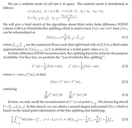
2 Spatial discretization

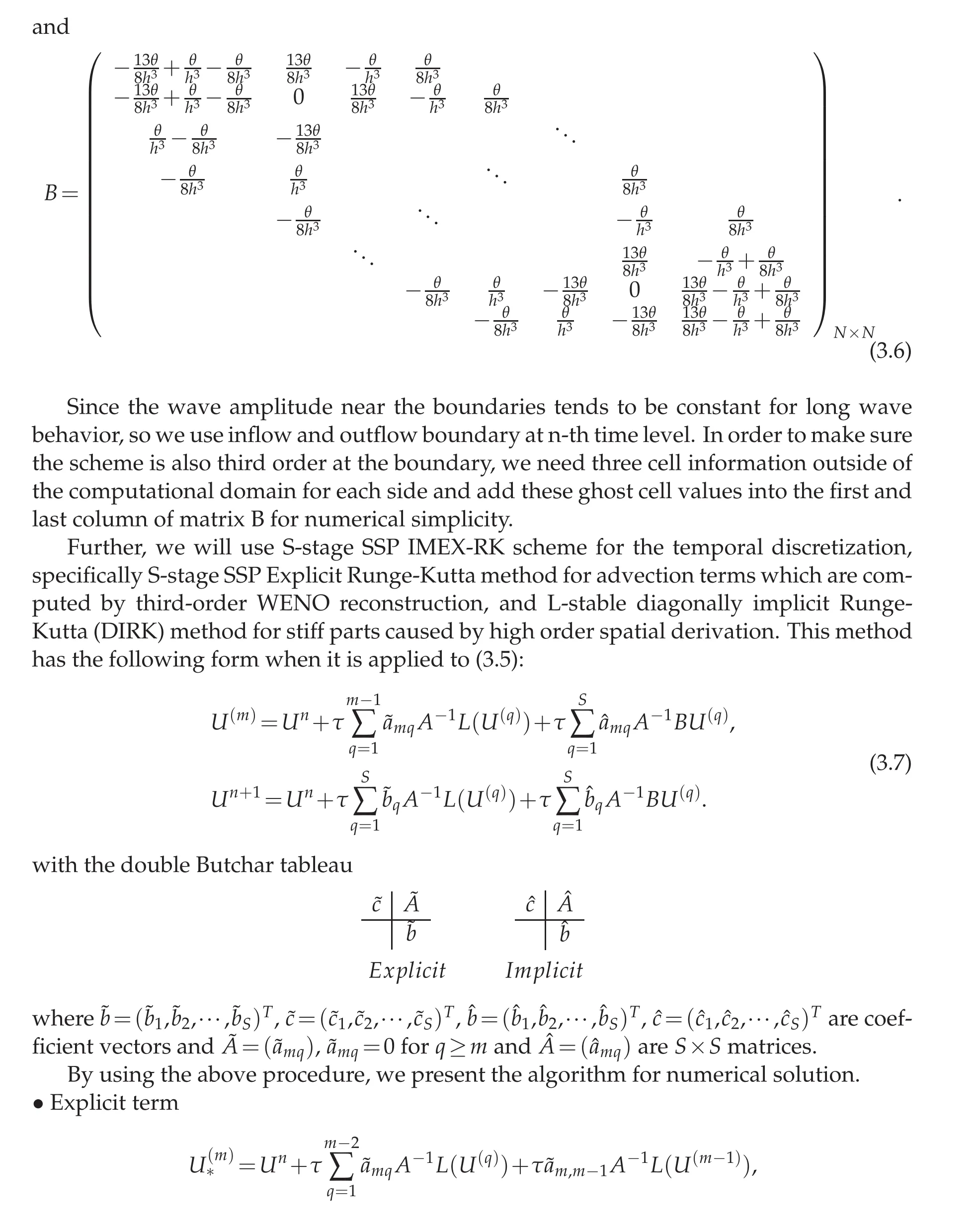
3 The third order SSP IMEX Runge-Kutta method

4 Numerical results

In this section,we will discuss computational results of the scheme(3.9)on some numerical examples for the solitary wave solution and shock wave solution of Rosenau-KdV equation and Rosenau-KdV-RLW equation.

wave velocity

and wave amplitude

Errors and rates of convergence in terms ofL1andL∞atT=20 forτ=CFL·hwithCFL=1 in intervalx∈[?70,100]are listed in Table 1 for Example 4.1.The third order accuracy of the numerical method is achieved as we expected in the theoretical procedure,and works well with large time step.We can observe from the left of Figure 1 that the solitary wave curve matches excellently with exact solution whenh=τ=0.1 atT=20.From the right of Figure 1,it can be seen that error mostly generates at two sides of the solidary wave.

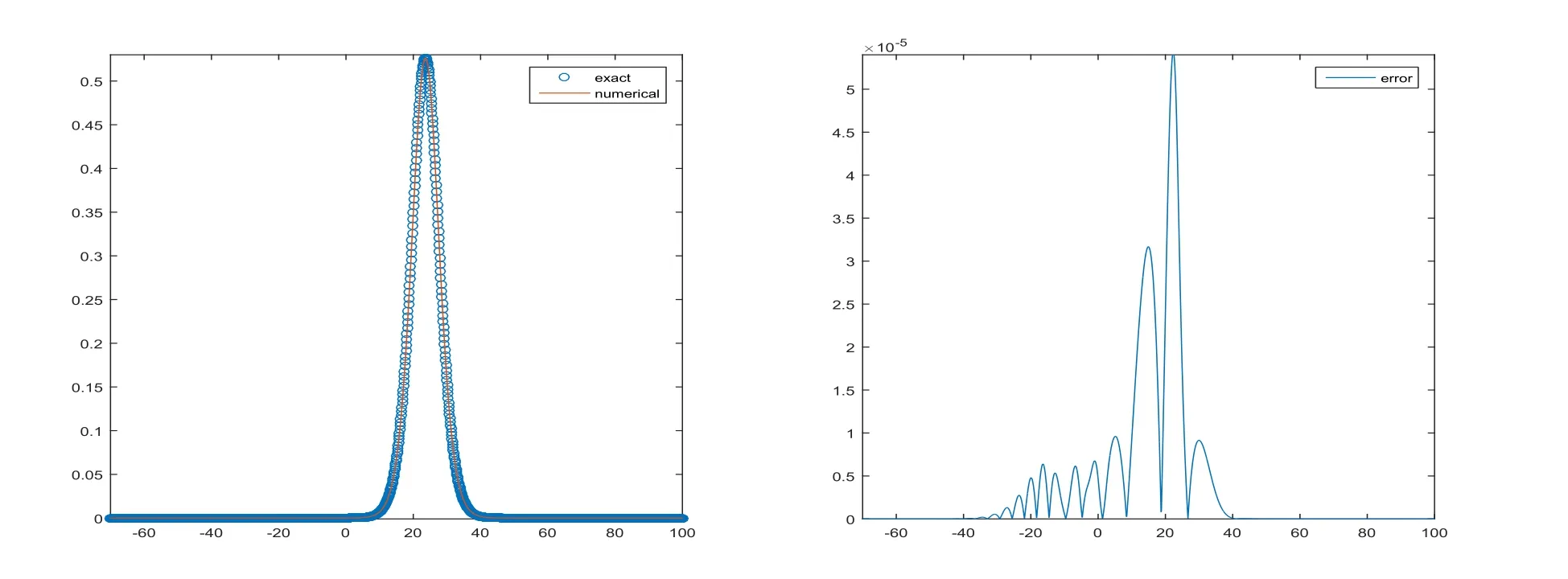
Figure 1:Wave graph of u(x,t)at T=20 and numerical solution of Rosenau-KdV equation with h=τ=0.1 at T=20(left)and error(right)for Example 4.1.

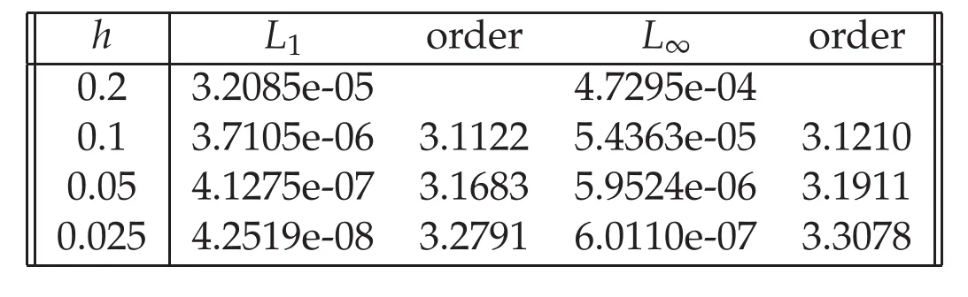
Table 1:Errors and rates of convergence when CFL=1,h=τ at T=20 for Example 4.1.

We compare theL∞errors of our scheme with the results of other three numerical schemes[11,12]under various mesh stepsh=τatT=20 in Table 2.The better computational accuracy of the present scheme can be seen with the smallest error among other schemes referred above.The solitary wave graphs atT=10,20 agree with the one atT=0 quite well.The solitary wave curve propagates with constant speed V to the right through time T in Figure 2.

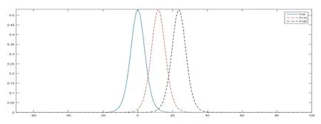
Figure 2:Numerical solution of Rosenau-KdV equation with h=τ=0.1 at T=0,10,20 for Example 4.1.]

Table 2:Comparison of L∞errors at T=20 for Example 4.1.

To observe the effect of power law nonlinear term to the solitary wave of Rosenau-KdV equation,we draw the wave curves forp=2,4,6,8,10 andwithh=τ=0.1 atT=20 in Figure 3,The wave amplitude and width are increasing whilepincreases.We computeL1,L∞errors forp=2,4,6,8,10 andatT=20 on three different meshes in Table 3 and also achieve third-order convergence in each case.

Figure 3:Numerical solution of Rosenau-KdV equation with p=2,4,6,8,10,?=and h=τ=0.1 at T=20 for Example 4.1.

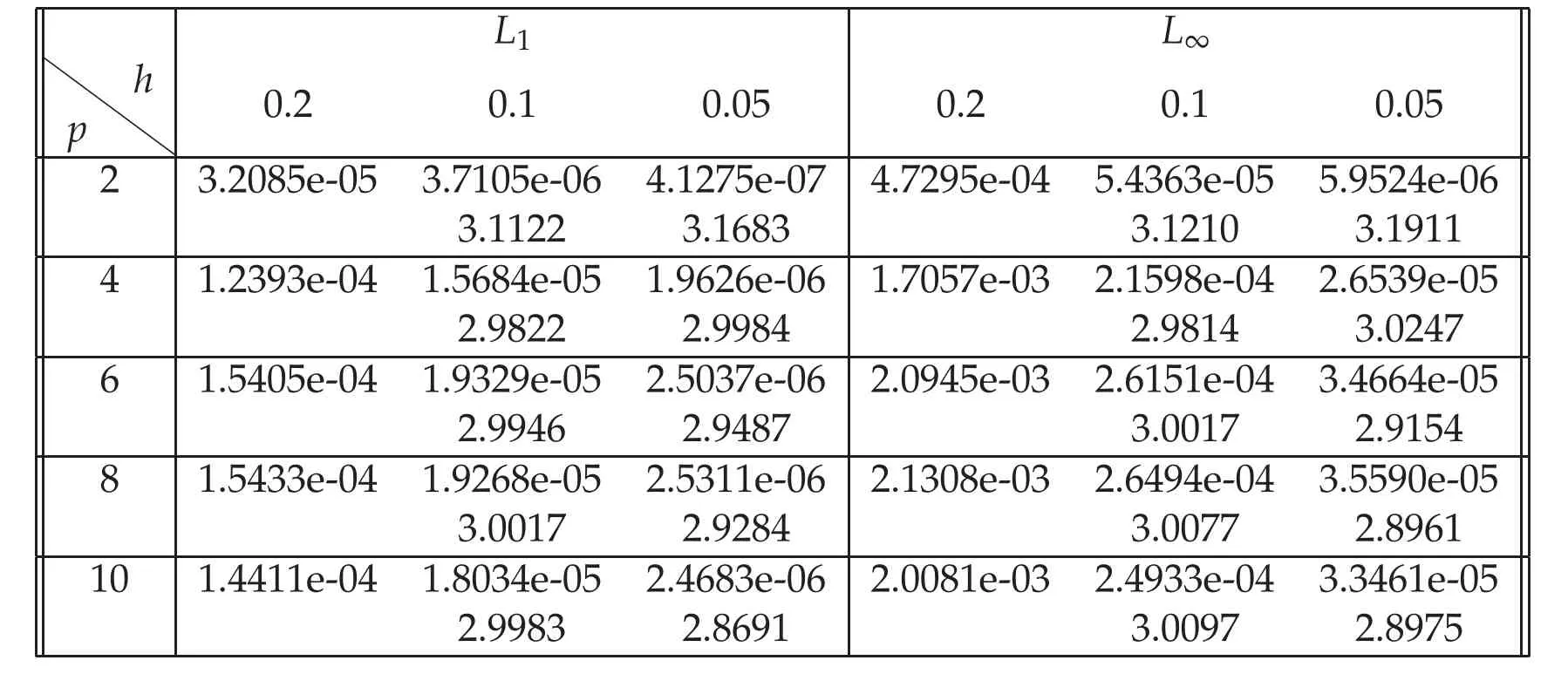
Table 3:L1,L∞ errors of numerical solutions for Rosenau-KdV equation with h=τ,T=20,ε=1pfor Example 4.1.

Next,we refer shock wave solutions of Rosenau-KdV equation from[3]which is available only for two particular values of power law nonlinearity parameterp=3,5.Our scheme simulates this wave phenomena efficiently with its essentially non-oscillatory property.

Example 4.2.Consider Rosenau-KdV equation(1.2)with parametersδ=0,ν= ?10,α=0.05,θ=0.001,?=?5,p=5:

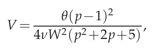
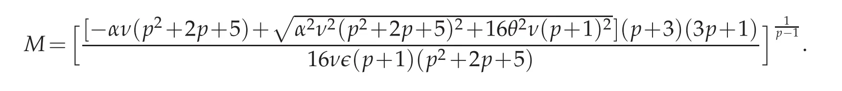
and choose the initial condition to beu0(x)=Mtanh(Wx),so that the analytical shock wave solution of Rosenau-KdV equation forp=5 isu(x,t)=Mtanh[W(x?Vt)]as in[3]with

These parameters have to be chosen carefully to make sure that the three quantities are all real.In Table 4,we show errors and rates of convergence to highlight the efficiency of the WENO reconstruction for shock wave in the case ofp=5.Figure 4 displays the shock wave atT=10 withh=τ=0.1 on the left and error on the right.As we can see there is no oscillatory nearby the stiff region.

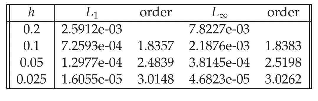
Table 4:Errors and rates of convergence when CFL=1,h=τ at T=10 for Example 4.2.

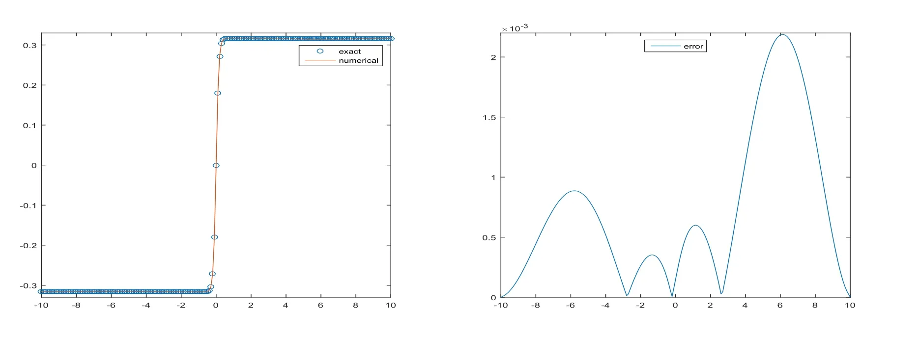
Figure 4:Wave graph of u(x,t)at T=10 and numerical solution of Rosenau-KdV equation with h=τ=0.1,p=5 at T=10(left)and error(right)for Example 4.2.

Example 4.3.Consider Rosenau-KdV equation(1.2)with parametersδ=0,ν= ?10,α=0.4,θ=0.01,?=?3,p=3:

and choose the initial condition to beu0(x)=Mtanh2(Wx),so that the analytical shock wave solution of Rosenau-KdV equation forp=3 isu(x,t)=Mtanh2[W(x?Vt)]as in[3]with

In Table 5,we give error and rate of convergence for shock wave whenp=3.Obviously here we achieve order that smaller than three at first,but it will converge to three eventually as the mesh is refined.Figure 5 displays the shock wave atT=10 whenh=τ=0.1 on the left and error on the right.

Table 5:Errors and rates of convergence when CFL=1,h=τ at T=10 for Example 4.3.

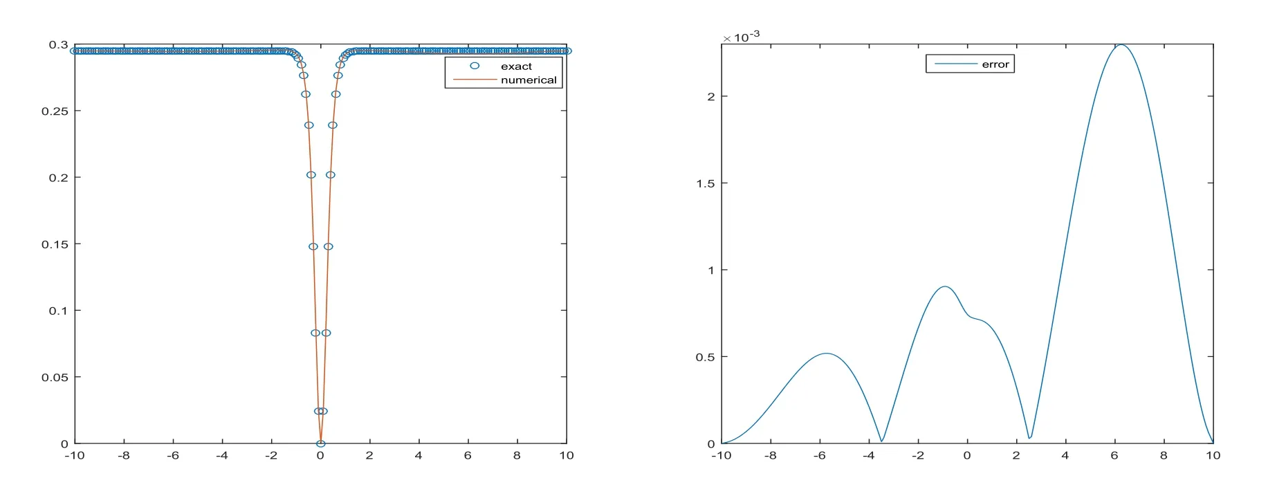
Figure 5:Wave graph of u(x,t)at T=10 and numerical solution of Rosenau-KdV equation with h=τ=0.1,p=3 at T=10(left)and error(right)for Example 4.3.

TheL∞errors of the numerical solutions atT=10 under various mesh stepsh=τare listed in Table 6 and compare with other three types of schemes studied earlier about the same equation,which shows that our scheme has the smallest error in any cases.

Table 6:The Comparison of L∞ errors with CFL=1,h=τ at T=10 between four different schemes for Example 4.4.

On the left of Figure 6,the numerical wave curve totally matches with the analytical solidary solution atT=10 with meshh=τ=0.1 over the intervalx∈[?40,60]and the corresponding distribution of the error is drawn for solitary wave in the right of Figure 6.

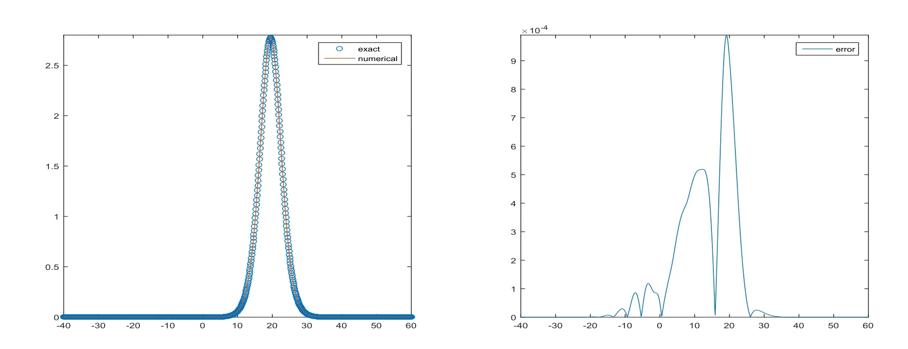
Figure 6:Wave graph of u(x,t)at T=10 and numerical solution of Rosenau-KdV-RLW equation with h=τ=0.1 at T=10(left)and error(right)for Example 4.4.

As shown in Table 7, the third-order convergence of the numerical solutions is verified atT=10 for the solitary wave problem of the Rosenau-KdV-RLW equation.In Figure 7,perspective views of the traveling solutions are graphed at various time levels forh=τ=0.1.

Table 7:Errors and rates of convergence with CFL=1,h=τ at T=10 for Example 4.4.

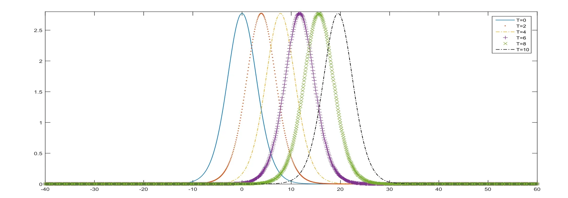
Figure 7:Numerical solution of Rosenau-KdV-RLW equation with h=τ=0.1 at T=2,4,6,8,10 for Example 4.4.

In order to observe the effect of power law nonlinear term to the solidary wave of Rosenau-KdV-RLW equation,TheL1,L∞errors and third-order convergence forp=2,4,6,8,10 andε=1/pon three different mesh are listed in Table 8.We draw the wave curves for thesepatT=10 withCFL=1,h=τ=0.1 andε=1/pin the intervalx∈[?40,60]for give further description in Figure 8.It can be observed that wave amplitude and speed decreases along withpincreases,this also fits the power law.

Figure 8:Numerical solution of Rosenau-KdV-RLW equation with p=2,4,6,8,10,?=and h=τ=0.1 at T=10 for Example 4.4.

Table 8:L1,L∞ errors of numerical solutions for Rosenau-KdV-RLW equation with h=τ,T=10,ε=for Example 4.4.

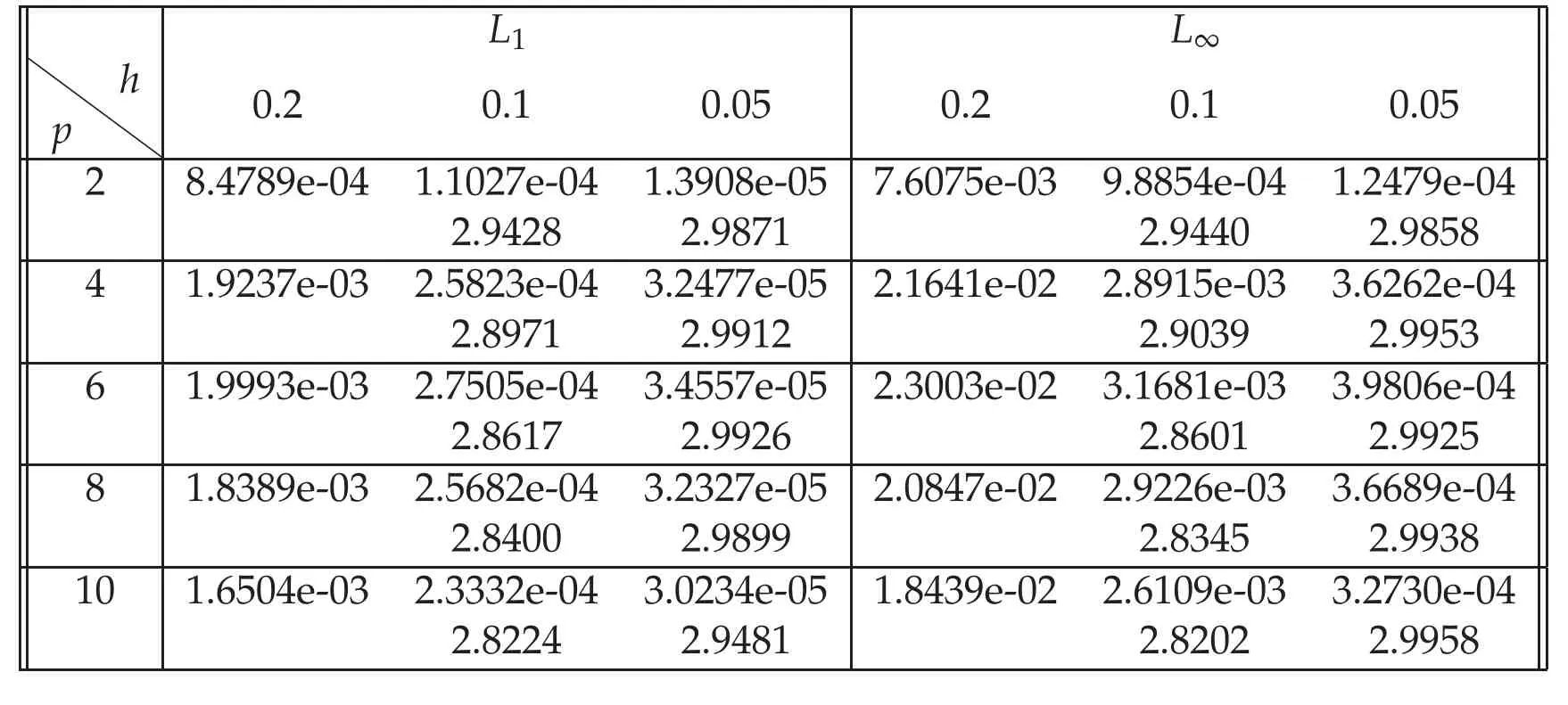
Table 8:L1,L∞ errors of numerical solutions for Rosenau-KdV-RLW equation with h=τ,T=10,ε=for Example 4.4.

L1 L∞p h 0.2 0.1 0.05 0.2 0.1 0.05 2 8.4789e-04 1.1027e-04 1.3908e-05 7.6075e-03 9.8854e-04 1.2479e-04 2.9428 2.9871 2.9440 2.9858 4 1.9237e-03 2.5823e-04 3.2477e-05 2.1641e-02 2.8915e-03 3.6262e-04 2.8971 2.9912 2.9039 2.9953 6 1.9993e-03 2.7505e-04 3.4557e-05 2.3003e-02 3.1681e-03 3.9806e-04 2.8617 2.9926 2.8601 2.9925 8 1.8389e-03 2.5682e-04 3.2327e-05 2.0847e-02 2.9226e-03 3.6689e-04 2.8400 2.9899 2.8345 2.9938 10 1.6504e-03 2.3332e-04 3.0234e-05 1.8439e-02 2.6109e-03 3.2730e-04 2.8224 2.9481 2.8202 2.9958

Based on earlier studies on the shock solution of the Rosenau-KdV equation,the shock wave solutions for the Rosenau-KdV-RLW equation were extracted by balancing principle only forp=3 andp=5 in[9].Here we will review related formulation for wave amplitude,width,velocity mentioned in[9,10],and then simulate both cases numerically as example.

Example 4.5.Consider Rosenau-KdV-RLW equation(1.3)with parametersδ=1,ν=?0.001,α=0.01,θ=0.001,ε=?1,p=3:

and choose the initial condition to beu0(x)=Mtanh2(Wx),so that the analytical shock wave solution of Rosenau-KdV-RLW equation forp=3 isu(x,t)=Mtanh2[W(x?Vt)]as in[9]with

In Table 9,the error comparisons inL∞,L1are obtained by present method for shock wave solution in the case ofp=3 of the Rosenau-KdV-RLW equation in intervalx∈[?10,10]withh=τ=0.2,0.1,0.05,0.025 respectively and the simulations are run up to timeT=10 to obtain the error norms.It can be easily found that the errors are small,and the third-order convergence of the numerical solutions are also verified.From Figure 9,we can catch the point that numerical solution fits with exact one,and numerical method approximate the exact solution even in stiff concave region successfully.

Table 9:Errors and rates of convergence with CFL=1,h=τ at T=10 for Example 4.5.

Figure 9:Wave graph of u(x,t)at T=10 and numerical solution of Rosenau-KdV-RLW equation with h=τ=0.1,p=3 at T=10(left)and error(right)for Example 4.5.

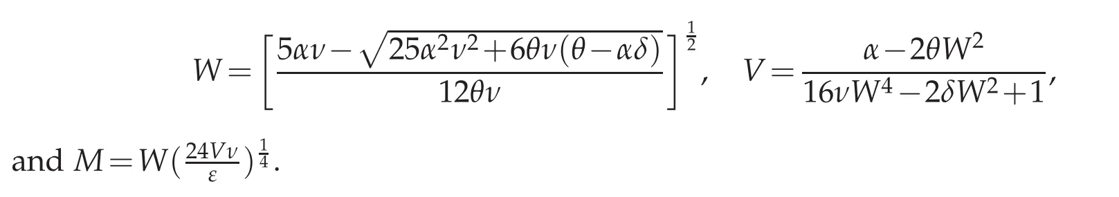
Example 4.6.Consider Rosenau-KdV-RLW equation(1.3)with parametersδ=1,ν=?10,α=0.05,θ=0.001,ε=?5,p=5:

and choose the initial condition to beu0(x)=Mtanh(Wx)so that the analytical shock wave solution of Rosenau-KdV-RLW equation forp=5 isu(x,t)=Mtanh[W(x?Vt)]as in[9]with

The computation of error and order is completed at timet=10 whenCFL=1,h=τon various mesh in intervalx∈[?10,10]and displayed in Table 10.The numerical shock wave curve of Rosenau-KdV-RLW equation forp=5 is agree with exact solution with no oscillatory near the pointx=0 whenh=τ=0.1 atT=10 on the left of Figure 10.

Table 10:Errors and rates of convergence with CFL=1,h=τ at T=10 for Example 4.6.

Figure 10:Wave graph of u(x,t)at T=10 and numerical solution of Rosenau-KdV-RLW equation with h=τ=0.1,p=5 at T=10(left)and error(right)for Example 4.6.

Example 4.7.Consider Rosenau-KdV-RLW equation(1.3)with parametersδ=?0.01,ν=0.01,α=0.01,θ=0.01,ε=1,p=3:

and Maxwellian initial condition to beu0(x)=exp(?0.005(x?60)2).

As a final example,we plot a high-frequency oscillatory behavior ofu(x,t)with above Maxwell initial condition in Figure 11 to illustrate the characteristic of dispersive shock wave behavior of(1.3).The steepening of the leading front repeats several times and decays until it is no longer present on the back of the wave.

Figure 11:Wave graph of Rosenau-KdV-RLW equation at T=0,5,10 with the Maxwellian initial condition u0=exp(?0.005(x?60)2)for Example 4.7.

5 Concluding Remark

To solve the solitary wave and shock wave problem of Rosenau-KdV equation and Rosenau-KdV-RLW equation,we use the third-order finite difference WENO reconstruction for advection terms,and central finite difference method for other terms in spatial discretization,then we use third-order SSP IMEX Runge-Kutta method for time discretization,in which the advection terms are treated by explicitly and remaining terms are treated by implicitly.In order to verify the effectiveness of the numerical scheme,some numerical examples are given for numerical experiment.Numerical simulations show that the method is very efficient with the advantages of non-oscillatory and looselyrestricted CFL condition.