Chao Yan(顏超) Jing Feng(馮徑) Ping-Lv Yang(楊平呂) and Si-Xun Huang(黃思訓(xùn))

1Institute of Meteorology and Oceanography,National University of Defense Technology,Changsha 410073,China

2State Key Laboratory of Satellite Ocean Environment Dynamics,Second Institute of Oceanography,State Oceanic Administration,Hangzhou 310012,China

3Basic Department,Nanjing Tech University,Pujiang Institute,Nanjing 211112,China

Keywords: mesoscale eddy,numerical differentiation,Tikhonov regularization,variational optimization analysis

1. Introduction

Mesoscale eddy refers to the widely distributed rotating water body in the ocean with diameters ranging from tens to hundreds of kilometers in spatial scale. It is easier to detect the horizontal velocity in the eddy motion and there has been a relatively large number of statistical laws.[1,2]The vertical velocity also plays an important role in the diagnosis and forecast of mesoscale eddy motion. As the vertical velocity in the oceanic large-scale motion is very small,which is only about one percent or one thousandth of the horizontal velocity[3,4]and cannot be easily measured directly by existing observation instruments, it can be diagnosed by other factors. For incompressible fluids,the horizontal velocityu,vand the vertical velocitywsatisfy the following continuity equation:

When the horizontal velocityu,vand upper and lower boundary conditions of the vertical velocity are known, the method of variational optimization analysis can be used to calculate the vertical velocity.[5,6]However there exist two problems:

Problem 1 The method involves the calculation of the divergence of(u,v). Ifu,vadopt the observation data ?u,?v,then on one hand ?u,?vare of low resolution because of sparse observation points,and on the other hand observational errors of ?u,?vwill bring about large errors of??u/?x,??v/?yafter differentiating ?u,?vby the finite difference method,and finally lead to a large error of the vertical velocity viaD=??u/?x+??v/?y.

Problem 2 The method needs vertical velocity boundary conditions to calculate the vertical velocity. In the field of Oceanography, it is difficult to precisely measure the vertical flow field at sea level.

Based on the above considerations, a new algorithm for reconstructing the three-dimensional flow field of the oceanic mesoscale eddy based on variation is proposed in this paper.Firstly, in order to reduce the effect of noise and enhance the resolution of the horizontal flow field,we make use of numerical differentiation technique on the observation data (?u,?v).The numerical differentiation[7,8]proposed in recent decades for inverse problems in mathematical physics has been widely used in atmospheric science and various fields.[9–12]It is shown that the method of numerical differentiation, based on Tikhonov regularization, is feasible to analyze meteorological observation data and improve the recognition rate of small and medium scale weather systems. Secondly,we modify the method of variational optimization analysis by calculating the vertical velocity at sea level from the known vertical velocity at the seafloor to obtain the vertical velocity boundary conditions. Furthermore,we employ simulation experiments to test the sensitivity of the new algorithm to observational errors and vertical velocity boundary conditions,comparing with the result of finite difference method. Finally, we reconstruct the vertical flow field for the real oceanic two-dimensional horizontal flow field data.

2. New algorithm:mathematical theory and calculation scheme

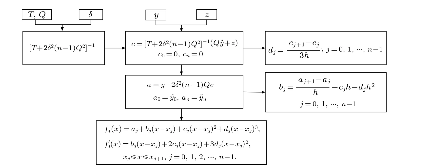
The overall calculating procedure is depicted as follows:

2.1. One-dimensional numerical differentiation

It is a typical ill-posed problem to calculate partial derivatives of the observation horizontal flow field(?u,?v)at each layer in mathematics,which can be overcome by making numerical differentiation on (?u,?v). The so-called numerical differentiation is to calculate the approximate derivative of a function with function values at some discrete points,also known as the differentiation on observation data. The main problem about the numerical differentiation is that it is not suitable because a tiny observational error may lead to a large error of the numerical result. In the atmosphere and ocean research community,we often need to calculate the directional derivative in the horizontal direction for the further calculation of dispersion and vorticity.The observational error may lead to great differences between the results obtained by the difference method and the differential method respectively. In recent decades, the most important method for making the numerical differentiation is the Tikhonov regularization.

(I)Raise the question

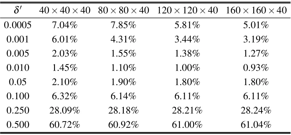
Supposey=y(x),x ∈[0,1],?={0=x0

1)|?yi ?y(xi)|≤δ,whereδis an observational error;

2) ?y0=y(0), ?yn=y(1).

Constructf?(x) from the observation data ?yi(i=1,2,...,n?1),maintaining a certain similarity betweenf′?(x)andy′(x)satisfying the following two conditions:

Here,αrepresents the regularizing parameter,f?(0)=y0and

f?(x)can be reconstructed by calculatingaj,bj,cjanddjas follows:

Remark 1 Since we obtain the cubic spline expression(4)of the functionf?(x)on each sub-interval,the observation field can be reconstructed and refined to any resolution.

It is required to find exact values ofy(x) atx=0 andx=1 for the calculation off?(x),which is impossible. Therefore, it is feasible to take ?y0, ?ynasy0,yn, with errors only atx=0,x=1,and takef?(x)on[x1,xn?1],in order to guarantee sufficient accuracy.

2.2. Reconstruct the vertical field from the horizontal flow field

Problem Assume that the observation flow field are ?u(x,y,z) and ?v(x,y,z), while the vertical observation data is unknown. The flow field area is set to be?×[0,H] and the analyzed flow field(u,v,w)is required to satisfy

Remark 2 For the ocean floor, it can be set asw0=0.ButwHcannot be observed generally,which is always handled aswH=?∫H0?Ddzapproximately.

3. Simulation experiment

In order to validate the effectiveness of the proposed algorithm, we first employ simulation experiments. Let?=[0,2π]×[0,2π]×[0,0.2π],(u,v,w)gives the real flow field Obviously?uT/?x+?vT/?y+?wT/?z=0.

Suppose that the observation horizontal flow field (?u,?v)is generated by adding a random error to the real flow field(uT,vT),which subjects to the uniform distribution on the interval[?δ,δ]. We employ the following four simulation experiments:

SchemeA1: Calculate the horizontal dispersion ?Dof the observation flow field by the finite difference method,and then obtain the vertical velocity by solving the equation?w/?z=??Dby the finite difference method.

SchemeA2: Calculate the horizontal dispersion ?Dof the observation flow field by the finite difference method, obtainλby solving Eq.(6),substitute it into Eq.(5)to produce(u,v),and finally calculate the vertical velocity by Eq.(7).

SchemeA3: Substitute the observation flow field with the reconstructed flow field,calculate the horizontal dispersion ?Dof the reconstructed flow field by the method of numerical differentiation, and then obtain the vertical velocity by solving the equation?w/?z=??Dby the finite difference method.

SchemeB: The implementation of the new algorithm.Substitute the observation flow field with the reconstructed flow field, calculate the horizontal dispersion ?Dof the reconstructed flow field by the method of numerical differentiation,obtainλby solving Eq.(6),substitute it into Eq.(5)to produce(u,v),and finally calculate the vertical velocity by Eq.(7).

Definition 1 The relative error between the vertical velocity and the real vertical velocity is defined as

3.1. Scheme comparison with definite δ

Conclusion 1 In the case of calculating derivatives with then same method,the method based on variation is superior to the traditional finite difference method for the vertical velocity calculation. Givenδ=0.05, Table 1 shows relative errors of calculation with different grid resolutions. The relative error of the schemeA2is much smaller than that of the schemeA1,and the relative error of the schemeBis much smaller than that of schemesA1,A2,A3.

Conclusion 2 The relative error of the schemeA1and schemeA2increases with the increment of resolution, while the relative error of the schemeBand schemeA3is almost unchanged, which further verified that the numerical differentiation is not suitable, and a small disturbance value of the observation flow field may lead to a large calculation error.

As seen from Table 1,the relative error of the schemeBis smaller than that of the schemeA2. When the grid resolution is 160×160×40, the relative error of the schemeBis 84%smaller than that of the schemeA2. The results show that for the vertical velocity calculation,the regularization method can effectively reduce the relative error compared with the method based on variation.

Table 1. Relative error of vertical velocity at different grid resolutions with δ =0.05.

In summary,the schemeBis the optimal scheme for calculating the vertical velocity. When the grid resolution is 160×160×40, the relative error of the schemeBis reduced by 91%compared with the traditional finite difference schemeA1,which means that the new algorithm is very effective.

3.2. Scheme comparison with unknown δ

Although the regularizing parameter is taken asα=δ2,the observational errorδis unknown in many practical situations. Therefore, it is necessary to test the calculation results of the schemeBaccording to the change of the presumed observational errorδ′. Suppose the true observational error isδ=0.05,and the regularizing parameter isα=δ′2.

Table 2 shows the relative error of vertical velocity obtained by the schemeBwith differentδ′. As can be seen from the table,even if the exact value ofδis unknown,the vertical velocity obtained by the new algorithm is still more accurate than that obtained by the finite difference method, as long asδ′is within a certain range. In some cases,such asδ′=0.010 andδ′=0.005,the relative error is smaller than that in the case ofδ′=δ=0.05. Therefore, according to the results shown in Table 2, as long asδ′is within the range of [0.01δ,2δ],the relative error of the schemeBis smaller than that of the schemeA1.

Table 2. Relative error of the scheme B with different δ′.

Fig.1. (a)The selected flow field and(b)the vector graph in this paper.

3.3. Scheme comparison without boundary conditions

The vertical velocity can be obtained by neither of the four methods when boundary conditions are unknown atz=0 andz=H. In many practical problems, it is difficult to obtain vertical velocity boundary conditions at both the top and the bottom. Therefore, it is necessary to solve the problem of missing boundary conditions when calculating the vertical velocity by the schemeA2or the schemeB. Assume that the vertical velocity atz=0 is known and the vertical velocity atz=His unknown. Then the following scheme can be taken to solve the problem.

SchemeB1Calculate the vertical velocity atz=Hby the schemeA3and take it as the boundary condition. Then recalculate the vertical velocity by the schemeB.

Whenδ=0.05, the vertical velocity atz=0.25πis not zero by Eq.(7).

As can be seen from Table 3,even the boundary condition is predicted by the finite difference method of the schemeB1,the variation-based method is still superior to the pure finite difference method of the schemeA3.

Table 3. Relative error without boundary condition with δ =0.05.

4. Reconstruction experiment on the vertical velocity of the oceanic mesoscale eddy

The experimental area is selected in 16.8750?N–21.8750?N,290.1250?–295.6250?W,depth of 5 m to 299.93 m below sea level (20 layers in total), as shown in Fig. 1(a).The horizontal oceanic data is sourcing from SODA(https://www2.atmos.umd.edu/ocean/) for January in 2001,SODA is the reanalysis data jointly released by the Department of Atmospheric and Oceanographic Sciences at the University of Maryland and the Department of Oceanography at TAMU,has a horizontal resolution of 0.25?×0.25?.

Fig.2. The distribution of vertical velocity at depth of 5 m,115.87 m,222.71 m and 299.93 m by the finite difference method with δ =0.15.

Fig.3. The distribution of vertical velocity at depth of 5 m,115.87 m,222.71 m and 299.93 m by the new algorithm with δ =0.15.

As seen from Fig. 1(a), there exists a mesoscale eddy in the region with a diameter of 70–100 km,the vector graph of the eddy is shown in Fig.1(b),it is a cyclonic eddy,and there is a strong south-to-north ocean current flowing into this eddy in the south,while the horizontal velocity is relatively slow in other’region except for a small eddy below left.

We use the new algorithm and the finite difference method respectively to calculate the vertical velocityw. Firstly, we take 299.93 m below sea level as the bottom layer. The vertical velocity of this layer is approximately 0 by analyzing the horizontal flow field of the layer and we can get the vertical velocity of the first layer,considered as the boundary condition,by further use of finite difference method. Based on the above boundary conditions, we take the observed data shown in Fig.1(b)as“real data”and discuss the new algorithm and the finite difference method respectively by introducing a disturbanceδ=0.15 as follows:

Fig.4. The vertical velocity profiles.

Fig.5. The position and the vector graph of an anticyclonic eddy.

Fig.6. The vertical velocity profiles of the anticyclonic eddy.

1) Calculate the vertical velocity at each layer by using the finite difference method with a small disturbanceδ=0.15.Figure 2 shows the distribution of vertical velocity at depth of 5 m,115.87 m,222.71 m and 299.93 m.

2) Calculate the vertical velocity at each layer by using the new algorithm proposed in this paper with a small disturbanceδ=0.15. Figure 3 shows the distribution of vertical velocity at depth of 5 m,115.87 m,222.71 m and 299.93 m.

Comparing Fig. 3 with Fig. 2, when the disturbance exists, the vertical velocity calculated by the new algorithm is more reasonable and feasible than that of the difference method. For the vertical velocity of mesoscale eddies, some parts rise,while some parts decline. The cause is related to the eddies surrounding environment, the phenomenon explained in the literature[14]is similar with our results.

The vertical velocity profiles of the flow field obtained by the two methods are shown in Fig. 4 (for display purposes,we multiply the value of the vertical velocity by 1000). The two figures on the top are profiles of vertical velocity obtained by the new algorithm, from longitude and latitude direction respectively. The two profiles at the bottom of Fig. 4 are obtained at the same longitude and latitude by the finite difference method. It can be seen from the profiles at the same position that the new algorithm is obviously better than the finite difference method.

Since the mesoscale eddy include cyclone and anticyclonic eddy, we have used the new algorithm to construct the three-dimensional flow field of cyclone eddy,similarly,we select an anticyclonic eddy and use the new algorithm to construct its three-dimensional flow field. As shown in Fig.5,the eddy located in the Cape of good hope,is an anticyclonic eddy.The horizontal oceanic data is also sourcing from SODA.

Based on the new algorithm,we calculate the vertical velocity of this anticyclonic eddy. The profiles of the vertical velocity are shown in Fig.6. It can be seen from the two profiles that there is a strong upwelling and a downwelling in this anticyclonic eddy,which is in line with the motion law of the fluid in the eddy.

5. Conclusion and perspectives

In this paper, a new algorithm for calculating the vertical velocity of the incompressible flow field based on variation is proposed. The partial derivative is calculated by using the one-dimensional numerical differentiation method based on Tikhonov regularization. Comparing with the traditional finite difference method, we can draw the following conclusions:

1) In the case of calculating derivatives with the same method,the method based on variation is superior to the traditional finite difference method for the vertical velocity calculation.

2) When the observational error exists in the horizontal flow field, the one-dimensional numerical differentiation method can effectively reduce the relative error of the vertical velocity.

3)In the case of an unknown observational error,the vertical velocity calculated by the new algorithm is still more accurate than that of the finite difference method if the ratio of the guess value to exact value is between 0.1 and 2.

4) The missing upper and lower boundary conditions of vertical velocity can be obtained approximately by the onedimensional numerical differentiation method and finite difference method. The relative error of vertical velocity recalculated by variation is also well controlled.

In summary, the vertical velocity calculation algorithm proposed in this paper is obviously better than the traditional finite difference method. This method can be widely used in the calculation of the vertical velocity in the ocean, meteorology and fluid experiment observations. Furthermore, by combining this method with the study of ocean dynamics and using the long-term data from SODA, the evolution of the three-dimensional structure of mesoscale eddies can be deeply studied.

Acknowledgments

The horizontal oceanic data used in this study are released by the SODA, which can be accessed in https://www2.atmos.umd.edu/ocean/. Inspired by the discussion with Wang Liang,the code of the proposed algorithm has been better optimized.