Tran Loc HUNG Phan Tri KIEN

University of Finance and Marketing,77 Nguyen Kiem Street,Phu Nhuan District,Ho Chi Minh City,Vietnam

E-mail:tlhung@ufm.edu.vn;phankien@ufm.edu.vn

Abstract The main purpose of this paper is to extend the Zolotarev’s problem concerning with geometric random sums to negative binomial random sums of independent identically distributed random variables.This extension is equivalent to describing all negative binomial in finitely divisible random variables and related results.Using Trotter-operator technique together with Zolotarev-distance’s ideality,some upper bounds of convergence rates of normalized negative binomial random sums(in the sense of convergence in distribution)to Gamma,generalized Laplace and generalized Linnik random variables are established.The obtained results are extension and generalization of several known results related to geometric random sums.

Key words Zolotarev’s problem;geometric random sum;negative binomial random sum;negative binomial in finitely divisibility;Trotter–operator technique

1 Introduction

An analogue of Zolotarev’s problem on geometric random sums originated by Klebanov et al.[12]is stated as follows:describe all random variables Y that for any p∈(0,1),there exists a random variable Xpsuch that

where?pis a Bernoulli random variable having probability mass function

In eq.(1.1)the random variables Y,Xpand?pare independent.In eq.(1.1)and from now on,the notationexpresses the equality in the sense of distributions.

The solution of eq.(1.1)is a geometric random sum,de fined as follows

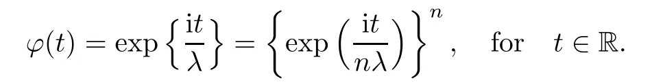
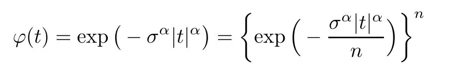
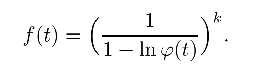
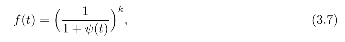
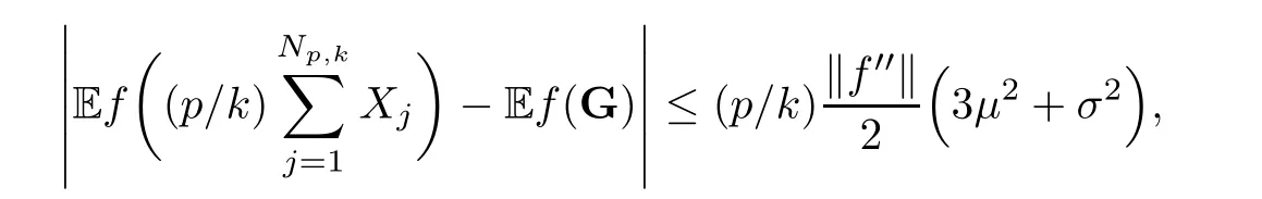
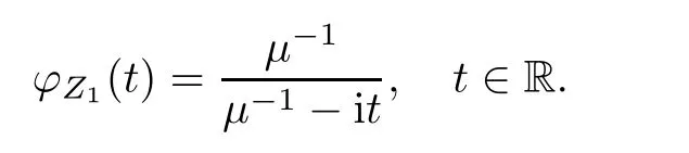
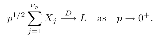
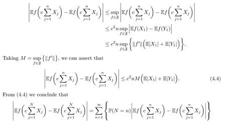
where Xp,j,j≥1 are independent,identically distributed(i.i.d.)random variables and νpis a geometric random variable with mean p?1,(0

Geometric random summations arise in many applied problems in physics,biology,economics,insurance mathematics,reliability,regenerative models,etc.Up to now,geometric random summations have been investigated by many authors like Klebanov et al.[12],Kruglov and Korolev[20],Kalashnikov[10],Sandhya and Pillai[25],Asmussen[2],Gnedenko and Kruglov[5],Lin[21],Kotz et al.[16],Kozubowski[18],Bon[3],Gamboa and Pamphile[4],Malinowski[23],Aly and Bouzar[1],Hung[6],and Korolev et al.[13–15],etc.

It is worth pointing out that the convolution of k(k∈N)geometric random variables with common parameter p,p∈(0,1)will be a negative binomial random variable with two parameters p∈(0,1)and k∈N(see for instance[27]).We propose here some natural enlargements of the class of geometrically in finitely divisible random variables is due to Klebanov et al.([12],De finition 1,page 792).Let Np,kbe a negative binomial distributed random variable with two parameters p∈(0,1)and k∈N,denoted by Np,k～NB(p,k),whose probability mass function de fined as follows

where x is an integer and x≥k(see[27],for more details).Recently,the negative binomial sums of i.i.d.random variables together with applications have been studies by Yakumiv[29],Sunklodas[27],Sheeja and Kumar[26],Jankovi′c[8],etc.It is clear that when k=1,the Np,1reduces to a geometric random variable νp～Geo(p),p∈(0,1).

For any p∈(0,1)and k∈N,let{Xp,k,j,j≥1}be a sequence of random variables,independent of Np,k.Consider the so-called negative binomial random sum

(see for instance[27]).It is plain that when k=1,the negative binomial random sum in(1.4)reduces to the geometric random sum de fined in(1.2).

By an argument analogous to result of Klebanov et al.[12],the negative binomial random sums in eq.(1.4)will be considered as an extension of Zolotarev’s problem.This extension is equivalent to describing all negative binomial in finitely divisible random variables and related results.Using Trotter–operator technique[28]together with Zolotarev-distance’s ideality,some upper bounds of convergence rates of normalized negative binomial random sums(in the sense of convergence in distribution)to Gamma,generalized Laplace and generalized Linnik random variables are established.Note that when k=1,the well known results related to weak limit theorems for geometric random sums will be obtained as direct consequences of theorems in this article.

This paper is organized as follows.Section 2 presents an extension of Zolotarev’s problem.Section 3 introduces the notion of a negative binomial in finitely divisible(NBID)random variable and related results.In Section 4,the accuracy of the approximations to the distributions of normalized negative binomial random sums are estimated.

2 An Extension of Zolotarev’s Problem

Let?pbe a Bernoulli random variable,de fined in eq.(1.1).The problem to be considered in this section is that of describing all random variablesYthat for any p∈(0,1)and k∈N,there are random variables Xp,kand Yjsuch that

and

where random variables Xp,k,Yjand?pare independent for j=1,2,···,k.

The following theorem will be considered as an extension of well-known result originated by Klebanov et al.in[12].

Theorem 2.1Let assumptions(2.1)and(2.2)hold.Then,the random variableYshould be de fined as a negative binomial random sum in the form

From(2.4)we conclude that

In the other hand,the relation(2.2)is equivalent to

Therefore,from(2.5)we have

It follows that

where Xp,k,jare i.i.d.copied of Xp,kand they are independent of Np,k～NB(p,k).

The proof is complete.

Remark 2.2When k=1,Theorem 2.1 reduces to Zolotarev’s problem in[12].

3 Negative Binomial In finitely Divisibility

The following notion will be needed in the sequel.

De finition 3.1A random variableYis said to be negative binomial in finitely divisible(NBID),if for any p∈(0,1)and for a fixed k∈N,there exists a sequence of i.i.d.random variables Xp,k,1,Xp,k,2,···such that

where Np,k～NB(p,k),and Xp,k,1,Xp,k,2,···are independent of Np,kand Y.

Remark 3.2The extension of Zolotarev’s problem,formulated in Section 2 is thus equivalent to describing all negative binomial in finitely divisible random variables.For a deeper discussion of de finition of negative binomial in finitely divisibility we refer the reader to[8]and[29].

Remark 3.3When k=1 the de finition of NBID random variables reduces to the well known de finition of geometric in finitely divisible(GID)random variables,originated by Klebanov et al.[12].Results of this nature may be found in[1,8,16,19,21,23].

The following theorem states that the weak limiting distribution of a negative binomial random summation is a NBID distribution.The symbolhereinafter denotes convergence in distribution.

Theorem 3.4For fixed k∈N,let

ThenYis a NBID random variable.

ProofLet us denote by fXp,k(t)the common characteristic function of Xp,k,jfor j≥1.According to[7](Theorem 9.1,page 193),the characteristic function of a negative-binomial random sumis given by

Thus,for fixed k,from(3.1),it follows that

where fY(t)is characteristic function of the limit random variableYand

It is clear that fk(t)is a characteristic function of limit distribution of a geometric random sum.

According to[20](Theorem 8.1.2,page 243),the characteristic function f(t)must be GID.

On the other hand,on account of Klebanov et al.[12](Theorem 2,page 792),it follows that

is an in finitely divisible characteristic function.Therefore,we get

where f(t)is an in finitely divisible characteristic function.

From Theorem 2.1 the proof is complete.

Remark 3.5It is worth noticing that the weak limit distribution of a geometric random sum will be GID distribution(see,for instance,[20],Theorem 8.1.2,page 243).It was deduced from Theorem 3.4 for case of k=1.

Theorem 3.6A random variableYis NBID if and only if its characteristic function fY(t)is given by

where ?(t)is a characteristic function of some in finitely divisible(ID)distribution.

ProofWe first observe that,on account of Theorem 2.1,the random variableYis NBID if and only if both relations(2.1)and(2.2)hold.Evidently,the relation(2.1)holds if and only if all random variables Yj,j=1,2,···,k are geometrically in finitely divisible(see[12]for more details).According to Theorem 2 in[12],it follows that

where ?(t)is an in finitely divisible characteristic function.

In the other hand,the relation(2.2)is equivalent to

According to(3.3),we conclude that,the random variableYis NBID if and only if

where ?(t)is an in finitely divisible characteristic function.The proof is complete.

Remark 3.7The similar result is due to Jankovi[8]and Yakumiv[29]with de finition of negative binomial in finitely divisible random variable in the form

Remark 3.8When k=1,the relation(3.1)reduces to geometric in finitely divisible(GID)characteristic function that is

where ?(t)is an in finitely divisible characteristic function(see[12],Theorem 2,page 792).Result of this nature also may be found in[20](Theorem 8.1.1,pages 241–242).

Corollary 3.9(The Lvy–Khinchin type representation) A random variableYis NBID if and only if its characteristic function is given in the form

where k∈N and γ is a real constant,G(x)is a bounded non-decreasing function.Note that the function under the integral sign is equal to?t2/2 at the point x=0.

ProofAccording to Lvy–Khinchin formula(see[24],page 30,Theorem 1.16),the function ?(t)is an in finitely divisible characteristic function if and only if it admits the representation

On account of Theorem 3.6,the random variableYis NBID if and only if

Equivalently,

The proof is complete.

Remark 3.10When k=1,the relation(3.4)reduces to a geometric in finitely divisible(GID)characteristic function in form

(See[12],Corollary 1,page 792).

Some negative binomial in finitely divisible(NBID)random variables are shown as follows.

Example 3.11LetGbe a Gamma distributed random variable with two parameters λ>0 and k∈N,denoted byG～Gamma(λ,k),whose characteristic function is given by

It is clear thatGis a negative binomial in finitely divisible random variable.Indeed,we have

Therefore,?(t)is an in finitely divisible characteristic function.By Theorem 3.4,we get the con firmation.

According to[16],a random variable L is said to be classical Laplace distributed random variable with parameters zero and σ>0,denoted by L～Laplace(0,σ),if its characteristic function has the form

Let L1,L2,···be a sequence of independent,classical Laplace distributed random variables with parameters zero and σ>0.For k∈N,write

Then,the characteristic function of L is given by

Extending the concept of classical Laplace distributed random variable,the generalized Laplace distributed random variable will be introduced as follows.

De finition 3.12A random variable L is said to have generalized Laplace distribution,denoted by L～GLaplace(0,σ,k),if its characteristic function is de fined by

For a deeper discussion of the generalized Laplace distributions and their properties we refer the reader to[9,11,13,16–18].

Remark 3.13When k=1,the generalized Laplace distributed random variable reduces to the classical Laplace distributed random variable with parameters zero and σ>0.

Example 3.14Let L～GLaplace(0,σ,k).Then,L is a NBID random variable.It is easily seen that for n∈N and t∈R,

is an in finitely divisible characteristic function.According to Theorem 3.6,we have the con firmation.

We follow the de finition used in[16].A random variable ξ is said to be symmetric Linnik distributed random variable with parameters α∈(0,2]and σ>0,denoted by ξ～Linnik(α,σ),if its characteristic function is given by

Lin[21]proved that Linnik distributions is geometric in finitely divisible(GID)and there are no closed–form expressions for the distribution and density function for Linnik random variable except for α=2,which corresponds to the Laplace distribution.

Let ξ1,ξ2,···be a sequence of independent,symmetric Linnik distributed random variables with parameters α∈(0,2]and σ>0.For any k∈N,set

Then,the characteristic function of ζ has following form

Extending the concept of symmetric Linnik distributed random variable,the generalized Linnik distributed random variable will be de fined as follows.

De finition 3.15A random variable ζ is said to have generalized Linnik distribution,denoted by ζ～GLinnik(α,σ,k),if its characteristic function is given by

For a deeper discussion of generalized Linnik distributions we refer reader to[11,13,16–18],and the references given there.

Remark 3.16When k=1,the generalized Linnik distribution reduces to symmetric Linnik distribution.Moreover,for k=1 and α=2,we obtain the classical Laplace distribution(see for instance[16]).

Example 3.17Let ζ～GLinnik(α,σ,k).Then,ζ is a NBID random variable.

For n∈N and t∈R,we have

is an in finitely divisible characteristic function.According to Theorem 3.6,we obtain the con firmation.

Theorem 3.18Let{fm(t),m=1,2,···}be a sequence of NBID characteristic functions converging to some characteristic function f(t).Then,f(t)is a NBID characteristic function.

ProofDue to{fm(t),m=1,2,···}is a sequence of NBID characteristic functions,according to Theorem 3.6,there exists a sequence of in finitely divisible characteristic functions{?m(t),m=1,2,···}such that

Letting m→∞,then fm(t)converges to the characteristic function f(t),hence ?m(t)will converge to the characteristic function ?(t),and

According to Lemma 1.20([24],page 30),?(t)is an in finitely divisible characteristic function.Therefore,on account of Theorem 3.6,it follows that f(t)is a NBID characteristic function.This completes the proof.

Remark 3.19When k=1,the Theorem 3.6 deduces to GID characteristic function as a limiting characteristic function of sequence of GID characteristic functions(see,for example,[12],Theorem 1,page 792).

Theorem 3.20Every NBID characteristic function is in finitely divisible.

ProofLet f(t)be a arbitrary NBID characteristic function.According to Theorem 3.6,we have

where ?(t)is an in finitely divisible characteristic function.It is plain that,

where ?(t)=e?ψ(t)is an in finitely divisible characteristic function.To complete the proof it remains to show that f(t)is an in finitely divisible characteristic function.

First,we attempt to show that

is an in finitely divisible characteristic function.According to Lukacs[22](Theorem 12.2.3,page 320),for any a>1 and g(t)is an arbitrary characteristic function,thenis an in finitely divisible characteristic function.For n≥1,taking

we have

On the other hand,by Taylor series expansion,we obtain

On account of Petrov[24](Lemma 1.20,page 30),the limit of a sequence of in finitely divisible characteristic functions is in finitely divisible.Therefore,the function h(t)is de fined by(3.8)is in finitely divisible.According to[22](Theorem 5.3.2,page 109),the characteristic function f(t)in(3.7),is the product of k in finitely divisible characteristic functions.Thus,f(t)is an in finitely divisible characteristic function.The proof is complete.

Remark 3.21It is to be noticed that every GID characteristic function is in finitely divisible(see,for instance,[20],page 242).It was deduced from Theorem 3.18 for k=1.

4 Bounds of the Accuracy of the Approximations to the Distributions of Negative Binomial Random Sums

We follow the notation used in[28].The symbol C(R)will denote the set of all bounded uniformly continuous functions on R with norm

Lemma 4.1Let{Xj,j≥1}and{Yj,j≥1}be two sequences of i.i.d.random variables with E|X1|r<+∞,E|Y1|r<+∞(r∈N).Assume that the following condition

holds for m=1,2,···,r?1(r∈N).Suppose that N is a positive integer–valued random variable,independent of all Xjand Yj(j≥1).Further,assume that E(N)<+∞.Then

where f∈Cr(R)and‖f(r)‖=

ProofUsing Taylor series expansion formula with Lagrange remainder for f∈Cr(R),we can assert that

where θ∈(0,1)and x∈R.From this,for X and Y are random variables and f∈Cr(R),we conclude that

Since|f(r)(x)|≤‖f(r)‖for any x∈R,from(4.1)it follows that

Based on Trotter–operator’s properties[28]and applying the inequality(4.2)to sequences{Xj,j≥1}and{Yj,j≥1}of i.i.d.random variables,we obtain

Let N be a positive integer–valued random variable,independent of all Xjand Yjfor j≥1,with E(N)<+∞.Then

The proof is complete.

Theorem 4.2Let X1,X2,···be a sequence of non–negative i.i.d.random variables with positive mean EX1=μ>0 and finite variance 0

where f∈C2(R).

ProofAccording to Example 3.11,theGis a NBID random variable.Let{Zj,j≥1}be a sequence of independent,exponential distributed random variables with parameterμ?1,independent of Np,k.It is easily seen that the characteristic function of random variables Zjis given by

According to[7](Theorem 9.1,page 193),the characteristic function of the negative-binomial sums(p/k)is de fined by

On account of the continuity theorem([7],Theorem 9.1,page 257),the Gamma distributed random variableGadmits the following presentation

It is immediate that

Applying Lemma 4.1 for r=2,we obtain

This completes the proof.

Remark 4.3The following results are direct consequences of Theorem 4.2.

1.Let k∈N be a fixed number.A limit theorem for negative binomial sums of i.i.d.random variables is stated as follows

Here and subsequently,the symbolstands for the convergence in distribution.

2.When k=1,the Gamma distributed random variableGreduces toEμ～Exp(μ?1),an exponential distributed random variable with meanμ>0.Then

where νp～Geo(p).Moreover,the R′enyi’s limit theorem for geometric sums of i.i.d.random variables(see e.g[20],Theorem 8.1.5,page 246)is stated as follows

Theorem 4.4Let{Xj,j≥1}be a sequence of i.i.d.random variables with EX1=0,E()=σ2and E|X1|3=.Let Np,k～NB(p,k),independent of all Xj,j≥1.Assume that L～GLaplacewith σ>0.Then

where f∈C3(R).

ProofOn account of Example 3.14,L～GLaplaceis a NBID random variable.Analysis similar to that in the proof of Theorem 4.2 shows that

where{Lj,j≥1}is a sequence of independent identically Laplace distributed random variables,independent of Np,k.It is clear that the characteristic function of Ljis given by

According to Kotz et al.([16],page 20),since L1～Laplace,it is a simple matter to

The proof is complete.

Remark 4.5As immediate consequences of Theorem 4.4,we have

1.For fixed k∈N the weak limit theorem for negative binomial sums of i.i.d.random variables is stated as follows

2.When k=1,then

It is worth pointing out that the Lemma 4.1 could not apply to the negative binomial sumsXj(0<α≤2),because its weak limiting distribution is Linnik law,whose absolute moments of order r are finite for 0

where x,y∈R.For any f∈F,we have the following lemma.

Lemma 4.6Let{Xj,j≥1}and{Yj,j≥1}be two sequences of i.i.d.random variables with E|X1|<+∞and E|Y1|<+∞.Assume that N is a positive integer-valued random variable,independent of all Xjand Yjfor j≥1.Assume that E(N)<+∞.Then,for any c0 and f∈F,there exists a positive constant M such that

ProofSince f∈F,one has by the Taylor series expansion

where 0<η<1 and x∈R.Since|f′(x)|≤‖f′‖for any x∈R and f∈F,for random variables X and Y with E|X|<+∞,E|Y|<+∞,we have

According to Zolotarev-distance’s ideality(see[30]for more details),from(4.3),we obtain

This completes the proof.

Theorem 4.7Let{Xj,j≥1}be a sequence of i.i.d.random variables with E|X1|=ρ<+∞.Assume that Np,k～NB(p,k),independent of all Xjfor j≥1.Then,for any f∈F,there exists a positive constant M such that

where ζ～GLinnik(α,σk?1/α,k)and 1<α<2.

ProofOn account of Example 3.17,ζ～GLinnik(α,σk?1/α,k)is a NBID random variable.Let{ξj,j≥1}be a sequence of independent,Linnik distributed random variables with two parameters σ>0 and α∈(0,2].It is obvious that the characteristic function of ξjis given by

Assume that Np,kis independent of all ξjfor j≥1.By an analogous to Theorem 4.2 we have

According to Kotz et al.([16],Proposition 4.3.18,p.212),since ξ1～Linnik(α,σ),we have

The proof is complete.

Remark 4.8Under the assumptions of Theorem 4.7 it follows that

1.Let k∈N be a fixed.Then

2.When k=1 we have

Moreover,the weak limit theorem for geometric random sum is stated as follows

Concluding remarksWe conclude this paper with the following comments.

1.In this paper,an extension of Zolotarev’s problem in[12]is discussed.The solution of the considered is a so-called negative binomial random sum that is equivalent to describing of negative binomial in finitely divisible(NBID)random variables.Some well known NBID distributions like Gamma,generalized Laplace and generalized Linnik distributions are shown as research examples.Estimate of convergence rates of normalized negative binomial random sums(in the sense of convergence in distribution)to Gamma,generalized Laplace and generalized Linnik random variables is also research objective of this article.The obtained results are extension and generalization of several known ones related to geometric random summations of i.i.d.random variables.The mathematical tool used in study of estimates of convergence rates is Trotter-operator technique together with Zolotarev-distance’s ideality.Some analogous notions and de finitions in this paper may be found in references[13–18].

2.An analogous result for the first point of Remark 4.7 is due to Korolev et al.in[13],using different way of proving.Theorem 6([13],page 13)is stated that

where Nn,ν～NB(1/n,ν),ν>0,independent of Xjfor j≥1.Note that the first parameter p of NB(p,ν)is taken as p=1/n and p→0+as n→∞.

3.The necessary and sufficient conditions of the convergence of distributions of random sums of i.i.d.random variables with finite variance to the Linnik distribution may be found in[14](Theorem 4,page 13)and[15](Theorem 4,page 9).

AcknowledgementsThe authors are greatly indebted to Professor Kozubowski,Tomaz J.from University of Nevada(US)for providing some his publications related to Geometric In finitely Divisible(GID)laws.