
THE INITIAL BOUNDARY VALUE PROBLEMS FOR A NONLINEAR INTEGRABLE EQUATION WITH 3×3 LAX PAIR ON THE FINITE INTERVAL?
2021-10-28 05:45:18YuXIAO肖羽
Yu XIAO(肖羽)
College of Information and Management Science,Henan Agricultural University,Zhengzhou 450046,China
E-mail:yuxiao5726@163.com
Jian XU(徐建)
College of Science,University of Shanghai for Science and Technology,Shanghai 200093,China
E-mail:jianxu@usst.edu.cn
Engui FAN(范恩貴)
School of Mathematical Science,Fudan University,Shanghai 200433,China
E-mail:faneg@fudan.edu.cn
Abstract In this paper,we apply Fokas uni fied method to study the initial boundary value(IBV)problems for nonlinear integrable equation with 3×3 Lax pair on the finite interval[0,L].The solution can be expressed by the solution of a 3×3 Riemann-Hilbert(RH)problem.The relevant jump matrices are written in terms of matrix-value spectral functions s(k),S(k),Sl(k),which are determined by initial data at t=0,boundary values at x=0 and boundary values at x=L,respectively.What’s more,since the eigenvalues of 3×3 coefficient matrix of k spectral parameter in Lax pair are three different values,search for the path of analytic functions in RH problem becomes a very interesting thing.
Key words integral equation;initial boundary value problems;Fokas uni fied method;Riemann-Hilbert problem
1 Introduction
Many physical phenomena(nonlinear optics and communication)can be reduced to solving nonlinear partial differential equations(PDEs).With the development of the real world,these phenomena are not only limited to the investigation of initial value problems,but also required some boundary conditions to be considered.Therefore,solving the initial boundary value problem of these equations is an important content in physical and optical communication and experimental research.
In 1997,Fokas[1]introduced the uni fied method for analyzing initial boundary value(IBV)problems for integrable nonlinear evolution PDEs,which further developed in[2]and[3].This method provides a generation of inverse scattering transform(IST)from initial value problem to IBV problem,it has been successfully used to analyze IBV for many of integrable equations with 2×2 lax pair such as the nonlinear Schr¨odinger(NLS)equation[4–6],the modi fied KdV[7,9],the Sine-Gordon[4,7],Camassa-Holm[10]equations and so on.In 2012,Lenells[11]developed this method for studying IBV problems for nonlinear integrable evolution equations on the half line with 3×3 Lax pair.Applying this method,IBV problems for nonlinear integrable evolution equations with 3×3 Lax pair on the half line were extensively studied such as Degasperis-Procesi equation[12],Sasa-Satsuma[13]and 3-wave[14]equations,and on the interval,there are some results that the two-component NLS[15],two-component Gerdjikov-Ivanov(GI)[16]and general coupled NLS[17].In 2017,Yan[18]extended this method for studying IBV problems for nonlinear spin-1 Gross-Pitaevskii equation with 4×4 Lax pair on the half line.After that,the spin-1 Gross-Pitaevskii equation[19]with 4×4 Lax pair on the interval was presented.
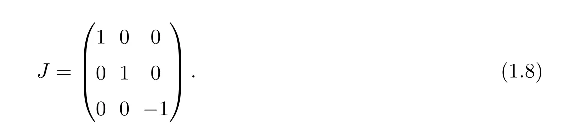
The nonlinear integrable system[11]
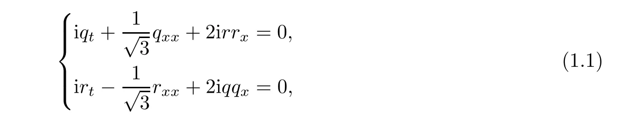

which is a reduction to the non-Abelian two-dimensional Toda chain.The system(1.1)is connected with the modi fied Boussinesq(mBsq)equation[22,23]that
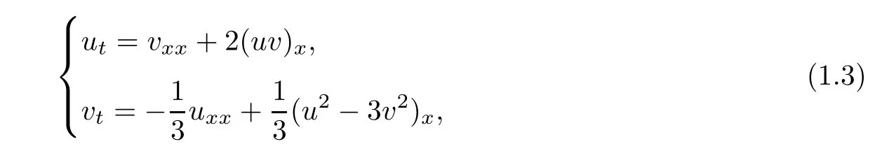
with u,v∈R,can be transformed into(1.4)under the transformation

In[21],the Darbooux transformation and in finitely many conservation laws of system(1.1)were investigated.In[11],lenells developed the uni fied method to analyzing IBV problems for integrable evolution equations with Lax pairs involving 3×3 matrices and extended this to system(1.1).
The purpose of this paper is to apply[3]and[11]to study the IBV problem of nonlinear integrable system(1.1)on the finite interval[0,L]with the IBV conditions that initial value:

and boundary value:
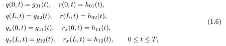
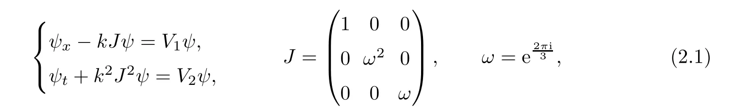
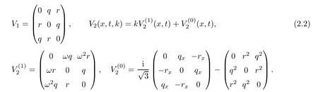
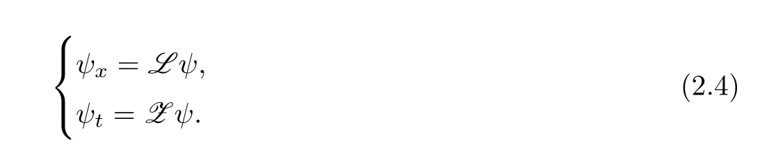
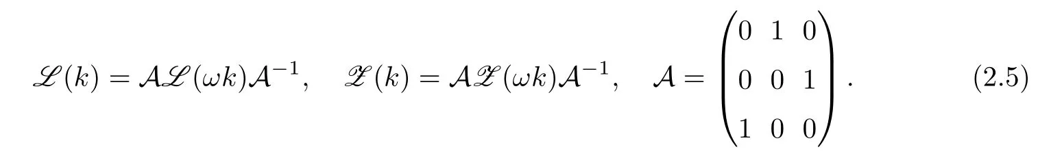
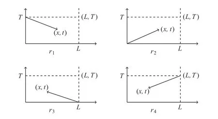
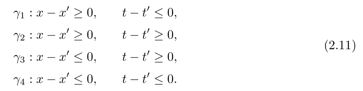
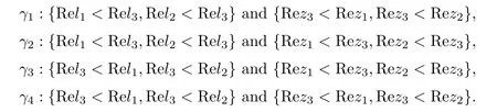
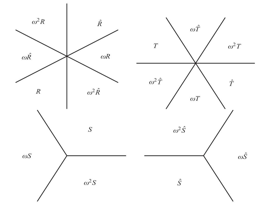
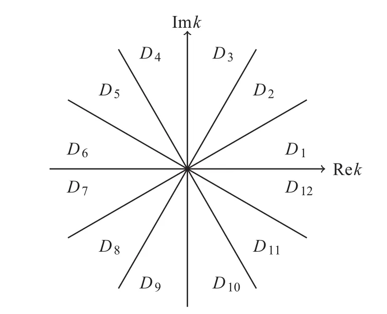
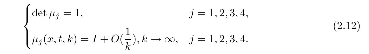
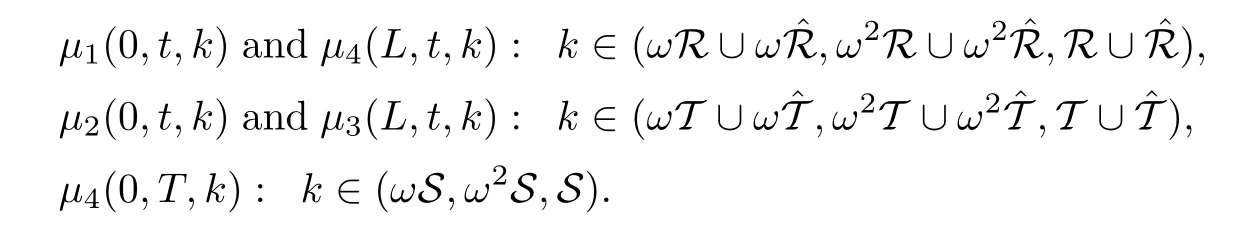
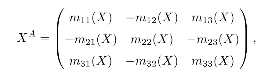
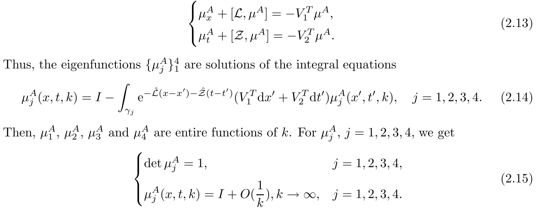
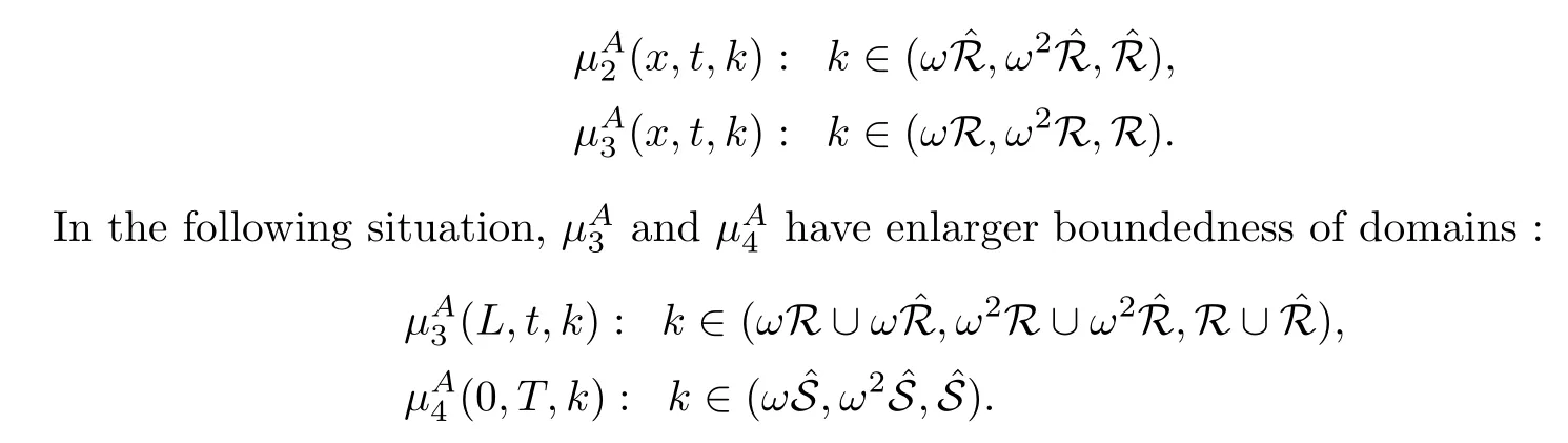
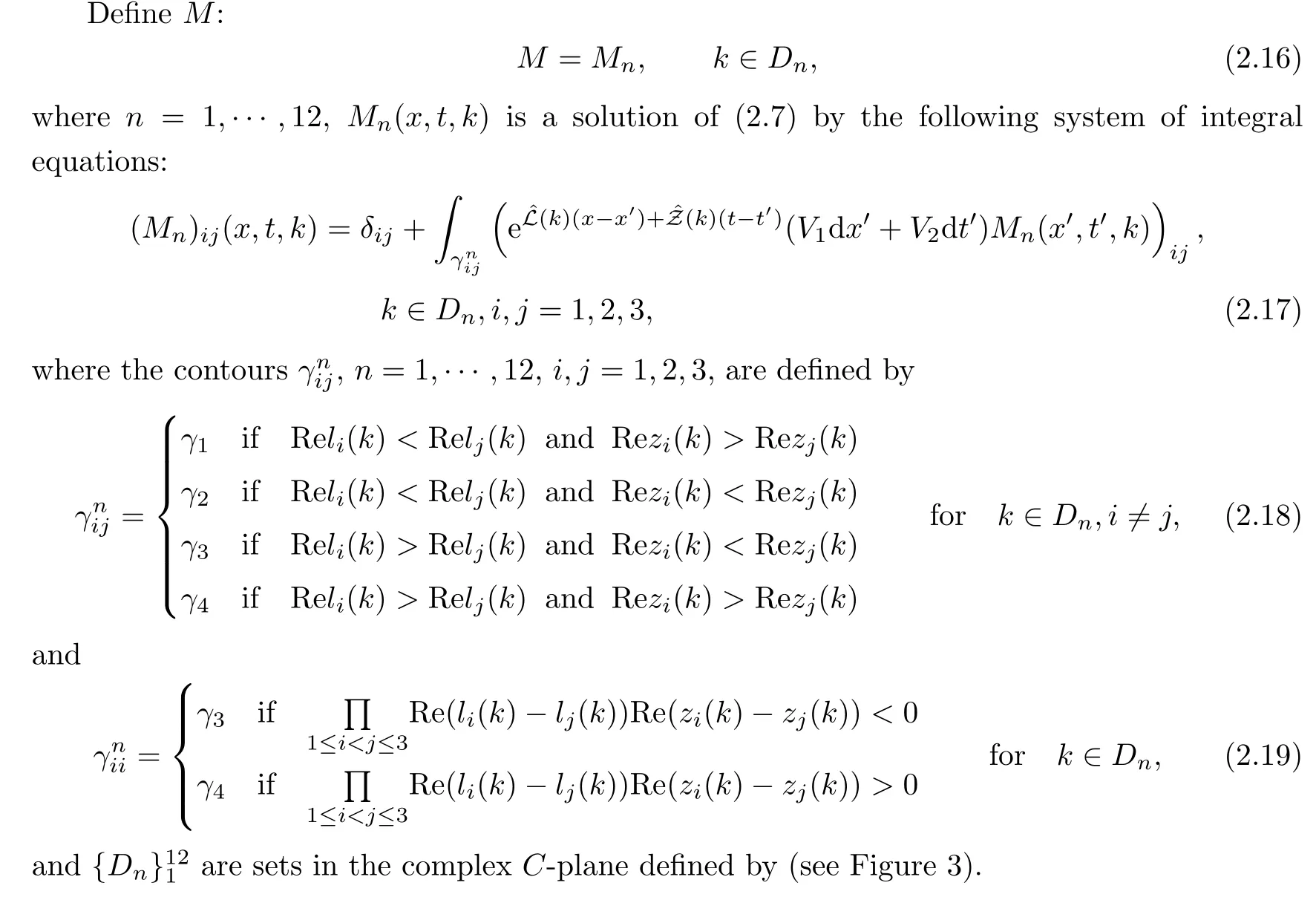
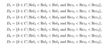
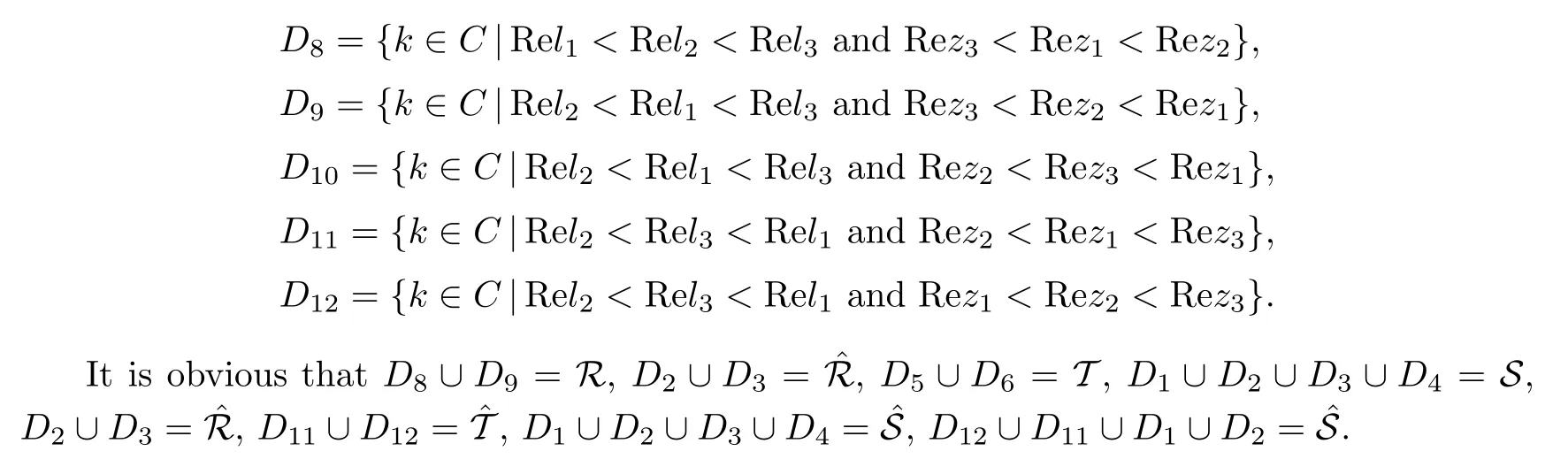
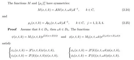
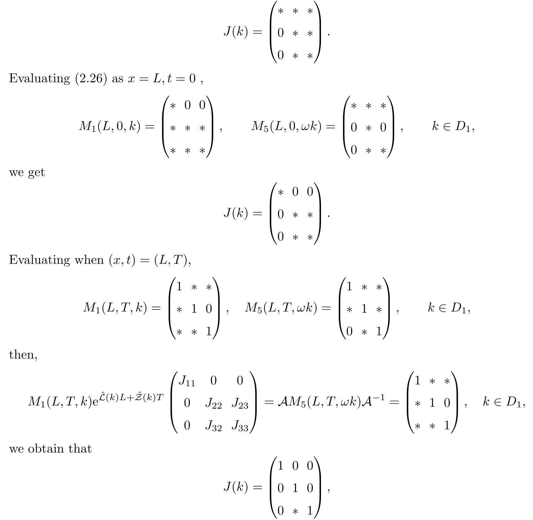
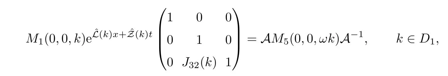
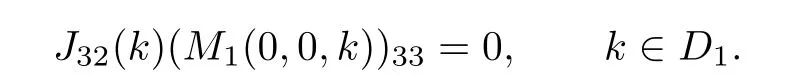
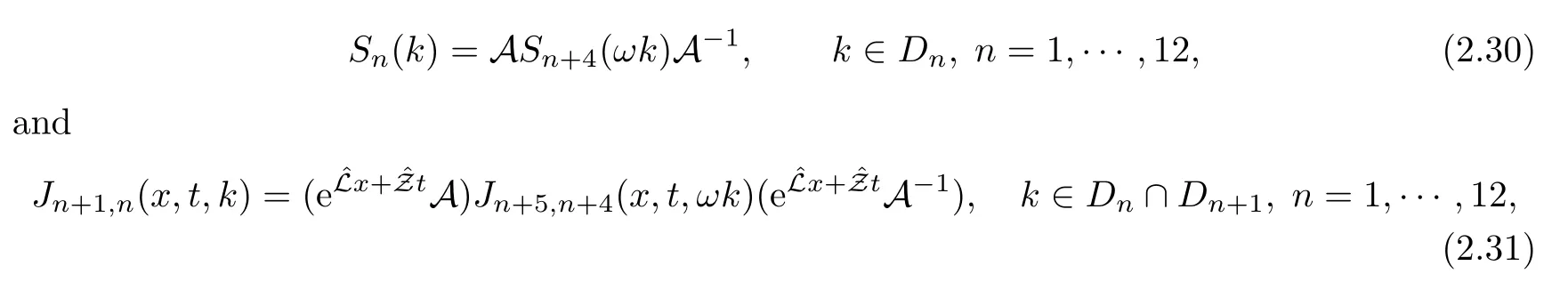
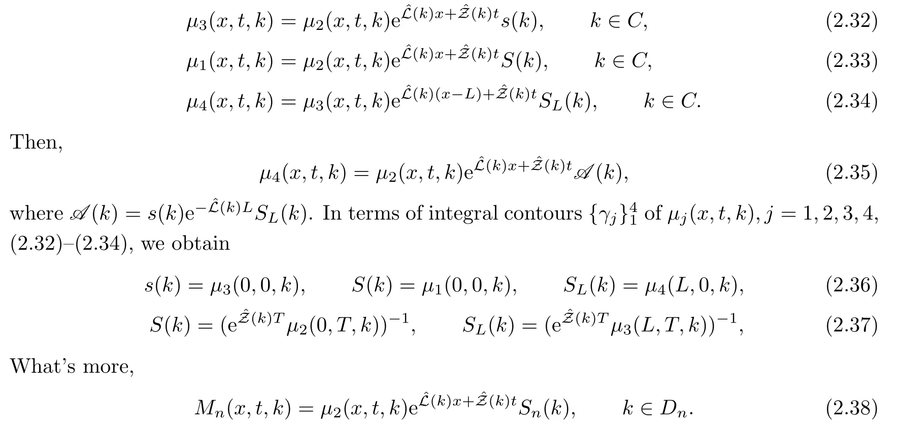
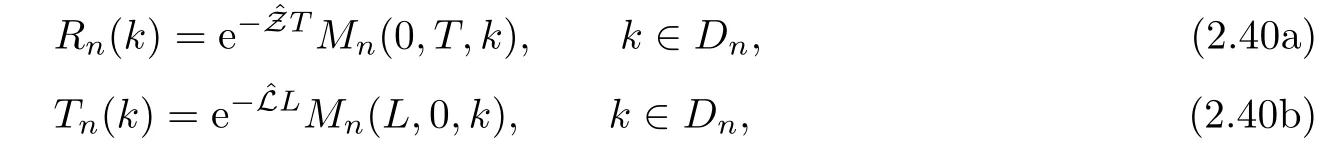
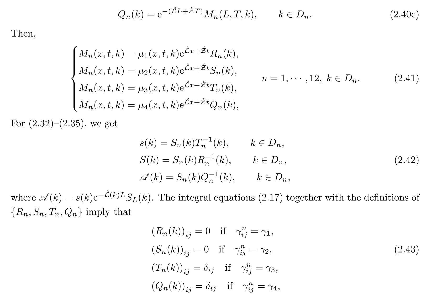
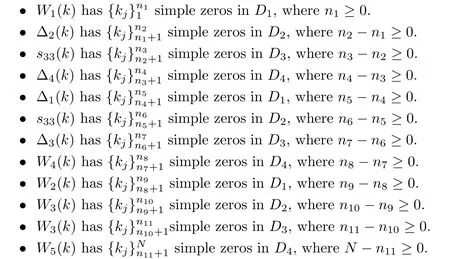
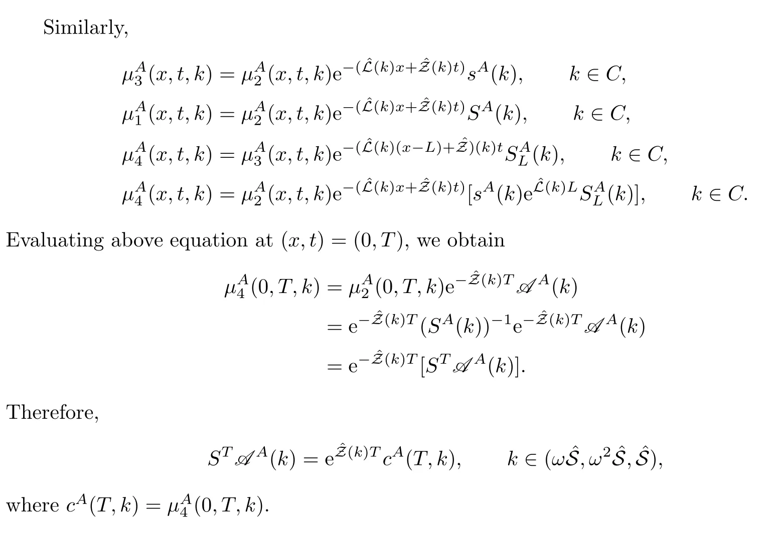
where q(x,t)and r(x,t)are complex-valued function for(x,t)∈?,? is denoted as ?={0≤x≤L,0≤t≤T}and 0 Dealing with the initial boundary problems for equation on the interval by uni fied method,there are some difficulties in getting the Riemann-Hilbert(RH)problem.The analysis here presents main distinctive difference:3×3 coefficient matrix of k spectral parameter in Lax pair: compared with[15–17], This paper is organized as follows.In Section 2,we discuss the eigenfunctions,spectral functions.According to them,we seek the conditions of a matrix RH problem.In this proceeding,there are two choices for the main diagonal paths of matrix RH problem,which depends on domain.In Section 3,we formulate the main RH problem,and the solution can be expressed by the formulated matrix RH problem. The system(1.1)has the Lax pair: where k is spectral parameter in complex C-plane,ψ(x,t,k),V(x,t)and V(x,t,k)are 3×3 matrix valued functions, L Z we can write(2.1)as L Z De fine Introducing a new eigenfunctionμ(x,t,k)by we can transform the Lax pair(2.4)into where W(x,t,k)is the closed one-form expressed by Figure 1 The r1,r2,r3and r4in the(x,t)-plane and The third column of the matrix equation(2.10)is related to exponentials By(2.11),they are bounded in the sets of complex C-plane: Also,the following functions are bounded and analytic for k∈C such that k belongs to Figure 2 The sets R,T,S and their re flections,, forms a complex C-plane Figure 3 The complex C-plane is composed of the sets Dn,n=1,···,12 It follows from(2.7)thatμ,μ,μandμare entire functions of k.Also,we can obtain In particular cases,μ,μ,μandμhave the larger boundedness of domains: Xshows the cofactor matrix of a 3×3 matrix X: where m(X)denotes(ij)th cofactor of X.By(2.7),the eigenfunctionμsatis fies the Lax pair Moreover,boundedness and analyticity is gotten: Proof We de fine spectral functions S(k),n=1,···,12,by Then M satis fies the jump conditions where the jump matrices satisfy It follows from(2.5),we get ψ(x,t,k)and Aφ(x,t,k)Asatisfy the same ordinary differential equation(ODE).Thus,there exists a matrix J(k) where?denotes an unknown functions.Combination of(2.28)and detM=1 in(2.20),(2.26)at(x,t)=(0,T)yields where J(k)=0 is not known element.Making use of the(x,t)=(0,0),equation(2.27)yields Using(2.29),evaluating the relation we deduce that Since J(k)is an analytic function and(M(0,0,k))→1 as k→∞for k∈D,we conclude that J=0 in D.This proves(2.24)for k∈D. It follows from(2.24),we obtain where the modulo of n is 12. De fine 3×3 matrix spectral functions s(k),S(k)and S(k)by A A Proof For the(2.38),M and S’s have same singularities.In terms of the 2.5 symmetries,we only need to study the singularities for k∈S.From formulas(2.39),the possible poles of M in S are as follows: and none of above zeros coincide.Also,we assume that all these functions have no zeros on the boundaries of the D’s. The spectral matrix functions s(k),S(k),S(k)have a relation so-called the global relation.Evaluating equation(2.35)at(x,t)=(0,T),we get Based on uni fied method,we can obtain the following result: Theorem 3.1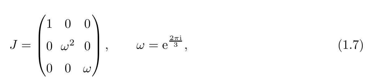

2 Spectral Analysis
2.1 A desired Lax pair
Introducing


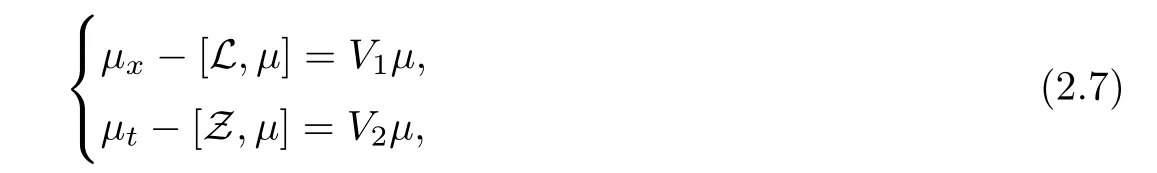


2.2 The analytic eigenfunctionsμj’s and their other forms


2.3 The Mn’s


2.4 The jump matrices


2.5 Symmetries


2.6 The relation of eigenfunctions
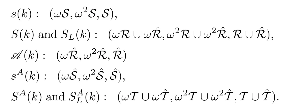
2.7 The spectral functions s
The spectral functions Sin(2.21)can be expressed in terms of the entries of s(k),S(k)and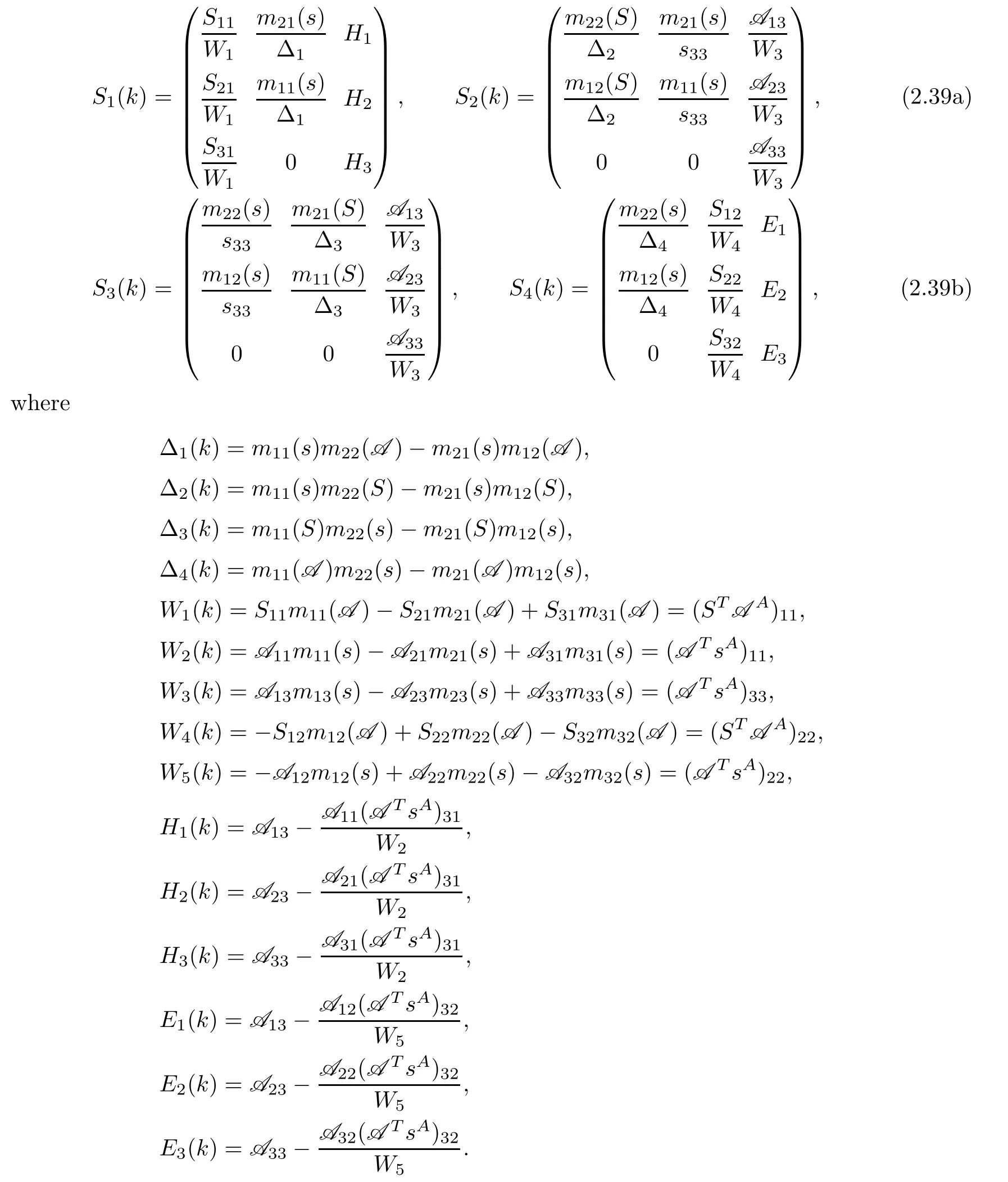


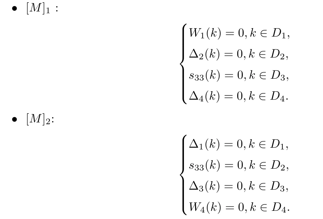
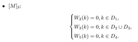
2.8 The residue conditions
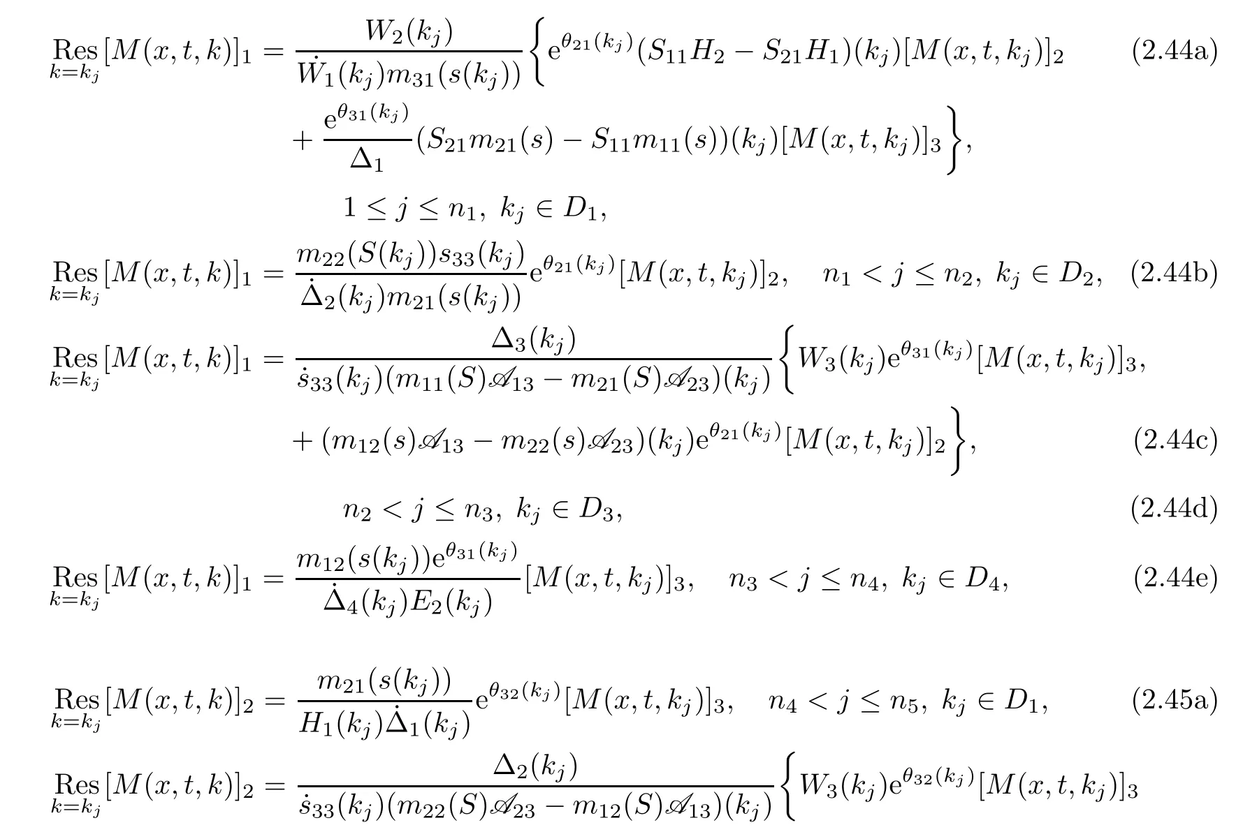
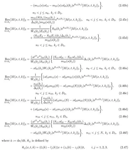
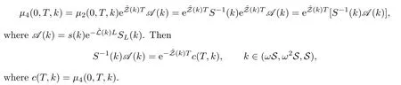
2.9 The global relation
3 The Riemann-Hilbert Problem
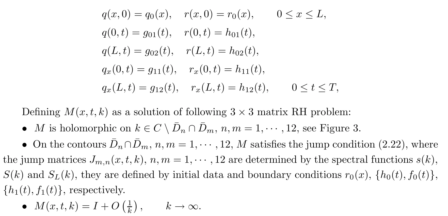
?M has simple poles kwith the part of(2.8)described and satis fies the associated residues conditions(2.44)–(2.46).For each zero kin S,there are two additional points,ωk,ωk,the associated residue conditions can be obtained from(2.44)–(2.46).
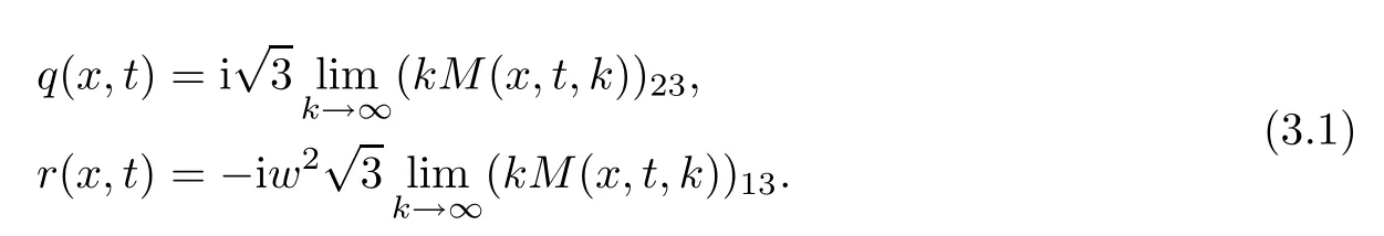
Then,M exists and is unique.What’more,the solution r(x,t)of equation(1.1)can be de fined by
Proof
It remains to prove(3.1)and this equation follows from the large k asymptotics of the eigenfunctions. Acta Mathematica Scientia(English Series)2021年5期
- Acta Mathematica Scientia(English Series)的其它文章
- THE UNIQUENESS OF THE LpMINKOWSKI PROBLEM FOR q-TORSIONAL RIGIDITY?
- HYERS–ULAM STABILITY OF SECOND-ORDER LINEAR DYNAMIC EQUATIONS ON TIME SCALES?
- ON NONCOERCIVE(p,q)-EQUATIONS?
- THE CONVERGENCE OF NONHOMOGENEOUS MARKOV CHAINS IN GENERAL STATE SPACES BY THE COUPLING METHOD?
- POSITIVE SOLUTIONS OF A NONLOCAL AND NONVARIATIONAL ELLIPTIC PROBLEM?
- A PENALTY FUNCTION METHOD FOR THE PRINCIPAL-AGENT PROBLEM WITH AN INFINITE NUMBER OF INCENTIVE-COMPATIBILITY CONSTRAINTS UNDER MORAL HAZARD?