
A modified Euler–Maclaurin formula in 1D and 2D with applications in statistical physics
2021-08-10 02:00:16JihongGuoandYunpengLiu
Jihong Guo and Yunpeng Liu
Department of Applied Physics,Tianjin University,Tianjin 300350,China
Abstract The Euler–Maclaurin summation formula is generalized to a modified form by expanding the periodic Bernoulli polynomials as its Fourier series and taking cuts,which includes both the Euler–Maclaurin summation formula and the Poisson summation formula as special cases.By making use of the modified formula,a possible numerical summation method is obtained and the remainder can be controlled.The modified formula is also generalized from one dimension to two dimensions.Approximate expressions of partition functions of a classical particle in square well in 1D and 2D and that of a quantum rotator are obtained with error estimation.
Keywords:summation technique,square well,quantum rotator,statistical physics
1.Introduction
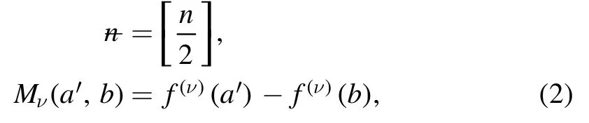
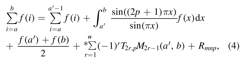
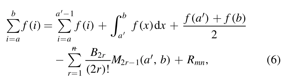
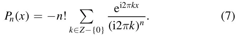
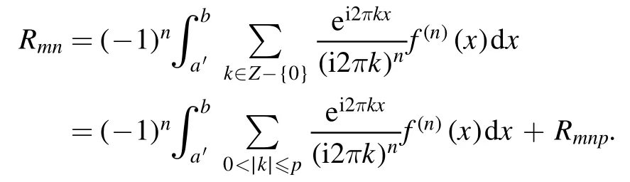
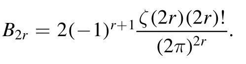
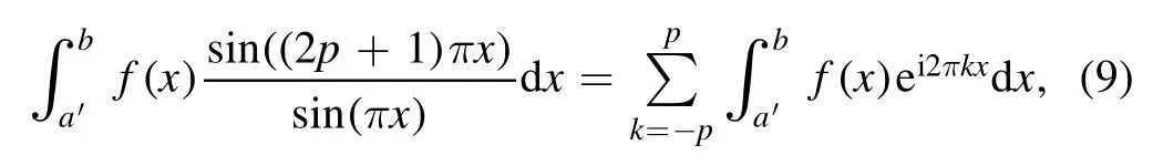
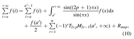
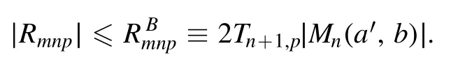
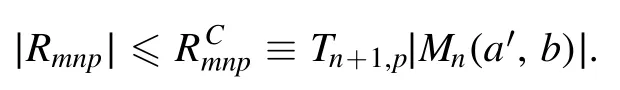
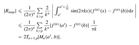
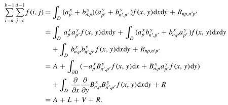
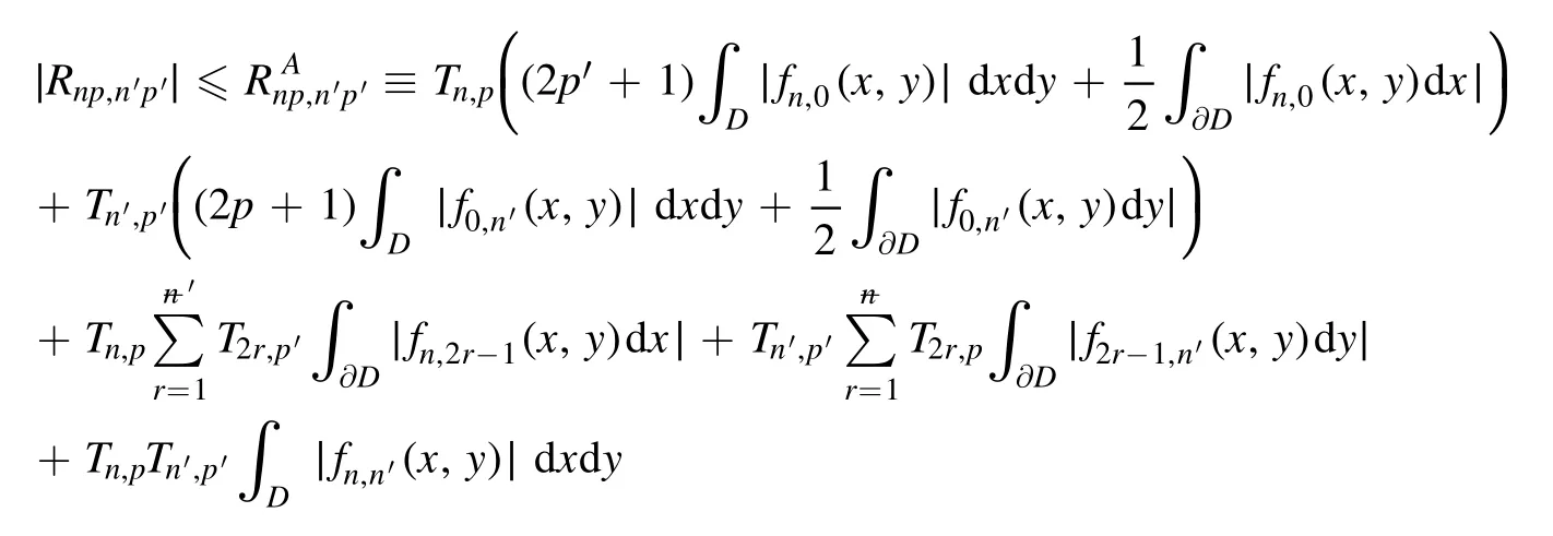
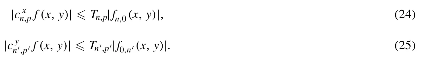
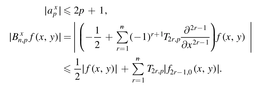
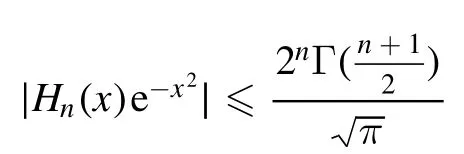
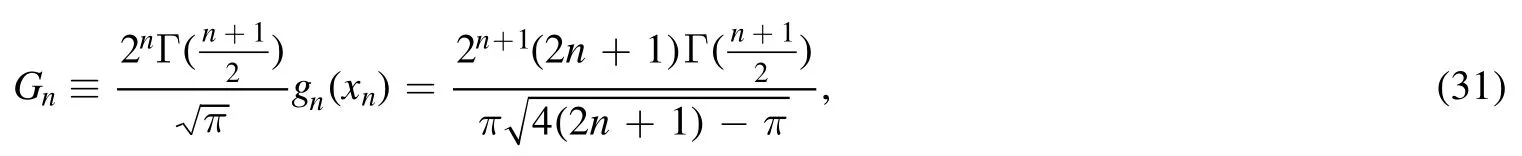
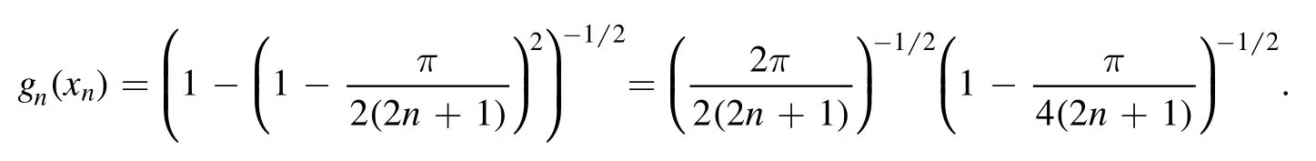
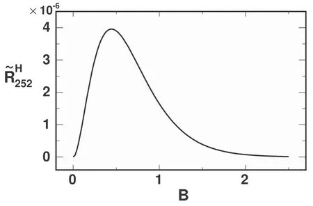
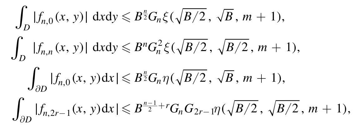
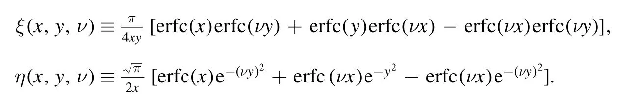
Summation is widely used in physics,especially in statistical physics.A traditional but powerful tool to work out a summation is the Euler–Maclaurin formula[1,2],which has lots of generalizations[3–5].If a real function f is Cnon an interval[a′,b]for some positive integer n and integersa′ Here B2rare the 2rth Bernoulli number and the symbols-nand M are defined as respectively,where the brakets in equation(2)and throughout stand for the floor function.The remainder term is with Pnbeing the periodic Bernoulli polynomial[6].Dropping the remainder term Rnin equation(1),one obtains an approximation of the summation on the left hand side.It is widely used for its high efficiency in most cases[7–9].However,as most asymptotic expansions,for givena′,band f,the remainder term usually does not converge to 0 as n→+∞.In our recent work[10],a modified Euler–Maclaurin formula(MEMF)was introduced to keep part of the remainder term in order to achieve higher accuracy.However,the MEMF was expressed rather technically than rigorously there.In this paper,we first review the MEMF in section 2 in a more rigorous way including an estimation of the upper limit of the remainder term,and then generalize the result to Dimension 2 in section 3.Some applications of the formulae in statistical physics are given in section 4. Theorem 1 MEMF in 1D.If a real function f is Cnon[a,b]for somen∈+Nand a,b∈Zwitha witha′=a+mandwhere the remainder term is Theζ(s)in the definition ofTs,pis the Riemann zeta function. proof.Two modifications are made to the original Euler–Maclaurin formula.(i)We sum over the first m terms explicitly,which is trival but necessary for some quantum systems at low temperature.(ii)We keep part of the original remainder in our calculations to improve the accuracy of the summation. We apply the Euler–Maclaurin formula to the summation on the left hand side after modification(i)and obtain witha′=a+m.The periodic Bernoulli polynomials of the remainder term in equation(3)can be expanded via Fourier series[11] Taking2pterms from the remainder term with∣k∣≤pin equation(7)and assigning the others to a new remainder term Rmnp,we have Using integration by parts,we have Note that Substituting equation(8)into(6),one obtains equation(4),and the proof is finished. Dropping the remainder term Rmnpin equation(4),an m-n-p cut of the MEMF is obtained,which can be used as an approximation of the summation on the left hand side.In practice,the integral in equation(4)can also be calculated by whose right hand side is a summation of Fourier coefficients of f on[a′,b].We remark that the integral kernelis identical to the multi-splits interference factor of an optical grating. Corollary 1.If the conditions in theorem 1 hold for allb>a′,and all the terms in equation(4)are finite asb→+∞,then with Obviously,similar conclusions can be drawn fora′=-∞,and for other results in this paper. Remark 1.We reveal the following connections to the Euler–Maclaurin formula and to the Poisson summation formula. 1.Takingm=0,p=0 in theorem 1,equation(4)becomes the original Euler–Maclaurin formula,that is equation(1). 2.Takingm=0,n=1 in theorem 1,if all the terms in equation(4)converges to finite values and R01pconverges to 0 asp→+∞,then with the help of equation(9),equation(4)becomes Furthermore,if all the terms in the above equation are finite and the summation on the left hand side converges asa→-∞andb→+∞,then it becomes the Poisson summation formula Theorem 2 Estimation of the remainder term.If the conditions in theorem 1 hold,then the remainder term Rmnpin equation(5)withn>1 can be controlled by the following estimations. 1. 2.If n is odd,andf(n)(x)is monotone with respect to x on[a′,b],then If n is even,andf(n)x()is monotone with respect to x on[a′,b],then proof. 1.Compute 2.For odd n,we estimate Note that the summation is an alternating summation,we have Similarly,for even n,we estimate Corollary 2.If the conditions in theorem 1 hold,and the interval[a′,b]can be divided intoNn-1subintervals on each of whichf(n-1)is monotone,then the remainder term in equation(4)withn>1 can be controlled as withΔMn-1=Mmax-Mmin,where Mmaxand Mminare the maximum and minimum values off(n-1)on[a′,b],respectively. Note that in theorem 1,the behavior of divergence is usually kept as n→+∞with fixed m and p,which only postpones the divergence.On the other hand,it converges as m→+∞or p→+∞with fixed n,which corresponds to the definition of the left hand side and a Fourier expansion of the original remainder term,respectively.In short,n is for efficiency,and m and p are for convergency. When the MEMF is used to work out a summation approximately,one first set a tolerance of error R*,and then choose some m and n according to the difficulty on calculating the right hand side other than the remainder term of equation(4).Next he estimatesor both Nn-1andΔMn-1,and then choose a p according to theorem 2 or corollary 2 to suppress|Rmnp|by the Tn,por Tn+1,pterm,so that it is not more than R*.Finally the right hand side other than Rmnpis calculated as an approximation of the left hand side with an satisfied error. Lemma 1 MEMF in a rectangle.Let D be the rectangle illustrated as in the left panel of figure 1,wherea,b,c,and d are integers satisfyinga with Figure 1.Summation points(left)in lemma 1 and the corresponding region D with its boundary(right). and the linear operators The operators with superscriptyare defined similarly.The factorsi,jin equation(14)is+1 for the vertices(a,c)and(b,d),while it is?1 for the vertices(a,d)and(b,c)as illustrated in the right panel of figure 1. proof.We rewrite equation(4)with m=0 as Applying the formula in equation(20)twice,it is easy to obtain That is equation(11). Note that(i)equation(11)holds for a single point,that is the case with b=a+1 and d=c+1,and(ii)all terms in equation(11)are additive with respect to the region D.If the region D is composed of several rectangles instead,equation(11)still holds,as long as si,jis properly redefined.This is the content of the next theorem. Theorem 3 MEMF in 2D.Suppose P is a set of integer pairs withP0?P,P1=P-P0,and Under the conditions of lemma 1,we have if all the terms are finite and well-defined,where A,L,V,and R are defined by equations(12)–(19),except thatsi,jis+1 if we turn from a vertical direction to a horizontal direction at(i,j)along the boundary?D,and it is?1 if we turn from a horizontal direction to a vertical direction at(i,j)along?D,such that the plus and minus signs appear alternately. Again,dropping the remainder term R,an approximation of the original summation in Dimension 2 is obtained. Theorem 4 Estimation of the remainder term in 2D.If f satisfies the conditions in theorem 3,then the remainder term in equation(22)[i.e.equation(15)]withn,n′>1 can be controlled by the following estimation proof.Equation(15)can be estimated by Note that,following the procedure in the proof of theorem 2,we have Thus, Note that Similarly, Thus theorem 4 holds. Obviously,for given n,n′and f,one can always choose proper p andp′to achieve as high accuracy as expected.Forn′=nandp′=p,the formula is simpler as follows. Corollary 3 Estimation of the remainder term withn=n′andp=p′.If f satisfies the conditions in theorem 3,then In this part,we give approximate expressions of partition functions in some simple systems by using the MEMF. 4.1.1.Partition function.For a one-dimensional infinite square well,the eigen energy is where?=?1is the eigen energy of the ground state.Thus the partition function withf(x)=e-Bx2and B=β?1.Then equation(10)gives with 4.1.2.Remainder estimation.It can be proved with the help of the integral representations of Hermite polynomials[12]that for allx∈Rand alln∈N,andHn(x)e-x2has at mostmonotonic intervals on[m+1,+∞),the remainder term can be controlled according to corollary 2 by for n>1. To have a better estimation of the remainder term,especially when m is large,we need a better estimation of Hn(x).Note thatis the(unnormalized)wave function of a quantum oscillator.By considering the classical corresponding of a quantum oscillator[13],we have the following conjecture Conjecture 1.An upper bound of Hermite polynomials can be estimated by with We have checked numerically that the conjecture holds at least for n≤20,and one can easily check given reasonable larger n numerically when necessary.As an illustration,the first 9 values of xnand gn(xn)are listed in table 1.If equation(29)holds,there is a rougher but simpler estimation: with for alln∈+N,since gn(x)increases as x increases at x>0,where we have inserted Then the remainder can be controlled according to corollary 2 by for n>1.The superscriptHhere and in the following implies that we have applied equation(30)which is based on Conjecture 1 on Hermite polynomials.From equation(32),it can be seen that when n is properly large,the remainder will be controlled for small B due to the power term,and when m is properly large,the remainder will be controlled for large B due to the exponential term,and when p is properly large,the remainder will be suppressed overall due to the effect of the Tn,pterm. Table 1.Approximate values of the first several xn and gn(xn). Table 2.Approximate values of [defined in equation(28)]with B=1. Table 2.Approximate values of [defined in equation(28)]with B=1. ? Table 3.Approximate values of defined in equation(32)]with B=1. Table 3.Approximate values of defined in equation(32)]with B=1. ? Therefore,one can easily make the remainder term as small as possible.We list some values of(defined in equation(28)),[defined in equation(32)]in table 2 and 3,respectively.It can be seen that the result can be as accurate as possible by choosing proper m,n,and p.If we regardas a function of B,the maximum is achieved atso that the remainder term can be controlled for all values of B.We plotas a function of B as an example in figure 2,where Bm=4/9.Therefore we have for all values of B.On the right hand side of equation(33),only the term Tn,pdepends on p,and it decreases to 0 as p→+∞.Thus with increasing p and fixed m and n,Zm+Wnp(m+1)is a series of functions with respect to B that converges uniformly to Z as a function with respect to B.Equation(29)can further be improved for large x,and we leave it for future work. 4.2.1.Partition function.For a quantum rotator,the eigen energy is with its degeneracy ωl=2l+1,and?1is the energy level of the first excited states.The partition function is given by Figure 2.The error bound[defined in equation(32)]as a function of B. 4.2.2.Remainder estimation.If equation(29)holds,then the remainder can be controlled through equation(30)according to corollary 2 as for n>1.Again,one can achieve given accuracy by choosing proper m,n,and p. 4.3.1.Partition function.We assume that a particle is in a two-dimensional infinite square well.Then the eigen energies are given by The partition function is with B=β?1,0.Applying theorem 3 to the above summation withP=+N2,P0={(i,j)∈P|i≤m,j≤m},P1=P-P0,n′=n,andp′=p,we obtain where Zmand Wnp(x)are defined in equations(26)and(27),see figure 3. 4.3.2.Remainder estimation.Now we try to give an upper bound of the remainder with the help of Conjecture 1.With the help of equation(30),we have forf(x,y)=e-B(x2+y2)andn1,n2∈N+.Note that f(x,y)=f(y,x).According to corollary 3,the remainder can be controlled by The four integrals above can be estimated by equations(37),(38)as with Therefore we have where n>1,p≥0,and m≥0.One can achieve any given accuracy by choosing m,n,p properly.Some values ofare listed in table 4. In this paper,a MEMF is introduced by working out part of the Fourier expansion of the remainder term in the original Euler–Maclaurin formula,which is also generalized to 2D.The MEMF includes both the original Euler–Maclaurin formula and the Poisson summation formula as special cases,and the remainder term of the MEMF can well be under control when the parameters m,n,p are properly chosen,so that it can be used as alternative way to work out a summation when the integral in the formula can be calculated.Approximate expressions of the partition functions of square well in 1D and 2D,and that of a quantum rotator are obtained with the help of the MEMF. Figure 3.Summation region of the partition function of a two-dimensional square well. Table 4.for square well with B=1 and m=0. Table 4.for square well with B=1 and m=0. n3579111315 p 0 2.2×10⁻² 4.7×10⁻³ 1.6×10⁻³ 7.2×10-44.0×10-42.6×10-42.0×10-4 1 5.8×10⁻³ 2.6×10⁻⁴ 2.1×10⁻⁵ 2.3×10-63.1×10-75.1×10-89.6×10-9 2 3.2×10⁻³ 5.8×10⁻⁵ 1.9×10⁻⁶ 9.0×10-85.3×10-93.8×10⁻¹⁰ 3.2×10⁻¹¹ 3 2.1×10⁻³ 2.1×10⁻⁵ 3.7×10⁻⁷ 9.5×10⁻⁹ 3.1×10⁻¹⁰ 1.2×10⁻¹¹ 5.7×10⁻¹³ 4 1.6×10⁻³ 9.7×10⁻⁶ 1.1×10⁻⁷ 1.7×10⁻⁹ 3.5×10⁻¹¹ 8.7×10⁻¹³ 2.6×10⁻¹⁴ Acknowledgments This work was supported by the‘Qinggu project’in Tianjin University under the Grant No.1701,and by the NSFC under the Grant No.s 11 547 043,11 705 125.We are grateful to Dr Wu-Sheng Dai,Dr Mi Xie,Dr Yong Zhang,Dr Kailiang Lin,and Dr Minghua Lin for helpful discussions. ORCID iDs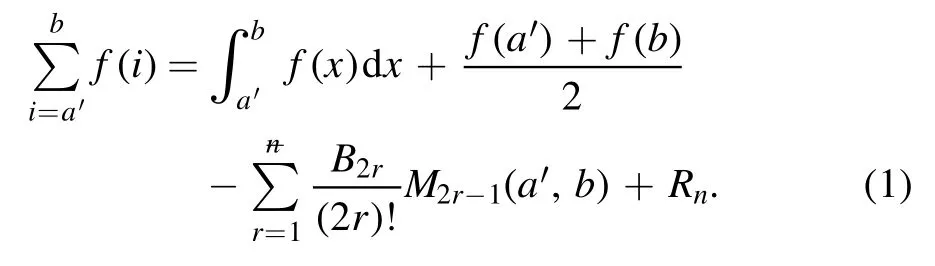

2.MEMF in Dimension 1


3.Generalization to Dimension 2


4.Applications
4.1.Partition function of a one-dimensional infinite square well


4.2.Partition function of a quantum rotator


4.3.Partition function of a two-dimensional infinite square well


5.Conclusion


 Communications in Theoretical Physics2021年7期