Zao Xu,Yin-Chenguang Lyu,Jiaozi Wang and Wen-Ge Wang

1 Department of Modern Physics,University of Science and Technology of China,Hefei 230026,China

2 CAS Key Laboratory of Microscale Magnetic Resonance,University of Science and Technology of China,Hefei 230026,China

Abstract We study the sensitivity of energy eigenstates to small perturbation in quantum integrable and chaotic systems.It is shown that the distribution of rescaled components of perturbed states in unperturbed basis exhibits qualitative difference in these two types of systems:being close to the Gaussian form in quantum chaotic systems,while,far from the Gaussian form in integrable systems.

Keywords:quantum chaos,sensitivity to perturbation,energy eigenstates,statistics

Introduction

Quantum manifestation of classical chaos is an important topic,which has been studied for several decades[1,2].Although manifestations in the spectral statistics have been studied well[3–7],not so much is known about wave functions,e.g.about statistical properties of energy eigenfunctions(EFs).In this paper,a new method is proposed and is shown capable of revealing interesting features of EFs of quantum chaotic systems.

Classical chaos refers to sensitivity of motion to initial condition; in Hamiltonian systems,this is equivalent to sensitivity to perturbation.Quantum mechanically,due to the unitarity of Schr?dinger evolution,quantum motion can not be sensitive to initial condition,while,it exhibits certain type of sensitivity to perturbation,measured by the so-called quantum Loschmidt echo(LE),or Peres fidelity[8].Loosely speaking,the LE decays exponentially in quantum chaotic systems under perturbations neither very weak nor very strong(see,e.g.[9,10]); here,under relatively strong perturbations,the decay rate is given by a Lyapunov-exponenttype quantity of the underlying classical dynamics[9].In contrast,in integrable systems,the LE shows a Gaussian decay within some initial times[11],followed by a power-law decay at long times[12].

One interesting question is whether stationary properties of quantum systems,particularly of their EFs,may exhibit some notable difference between integrable and chaotic systems under small perturbations.Intuitively,one may expect a positive answer.In fact,according to the semiclassical theory,the zeroth-order contribution to an EF from the phase-space motion is given by a uniform distribution in the classical energy surface for a chaotic system,meanwhile,in an integrable system,an EF resides around some tori[2,13,14].These two geometric structures in the phase space usually behave differently under small perturbations.

To find out a quantity that may measure the sensitivity of chaotic EFs to perturbation,one may start from the so-called Berry’s conjecture for EFs of quantum chaotic systems in the configuration space[13].Basically,the conjecture states that components of EFs in classically-energetically-allowed regions may be regarded as certain Gaussian random numbers.(Specific properties of the underlying classical dynamics may induce certain modifications to the conjecture[15–22].)Since components of integrable systems can not be regarded as Gaussian random numbers,it is natural to expect a notable difference between statistical properties of EFs in integrable and chaotic systems in the configuration space[23].

Berry’s conjecture is not written in a form that can be immediately used in the study of influence of small perturbation to statistical properties of EFs in unperturbed basis.To do this,one needs to consider components of EFs in classically-energetically-allowed regions of an integrable basis,which are rescaled by the averaged shape of the EFs,with the care of not taking average over the integrable basis states[24]; in quantum chaotic systems,this rescaling procedure leads to a Gaussian shape of the distribution of EF components.In this paper,we show that,under small perturbations,the distribution of rescaled components of perturbed EFs on unperturbed bases exhibit qualitatively different features in integrable and chaotic systems.

Analytical analysis

We use H0to denote the Hamiltonian of an unperturbed system.Its eigenstates are indicated by|k〉,with eigenenergiesin the increasing energy order,

Relatedly,a perturbed system’s Hamiltonian is written as

where ?V represents a weak perturbation with a small parameter ?.Eigenstates of H are denoted by |α〉,

with Eαalso in the increasing energy order.For the simplicity in discussion,we assume that both H0and H have a nondegenerate spectrum.

Components of the EFs of the perturbed states on the unperturbed basis are written as

For the simplicity in discussion,we consider only systems with the time-reversal symmetry,such that the components Cαkare real numbers.As shown in[24],for the purpose of studying statistical properties of EFs,one may consider rescaled components of Cαk,denoted by

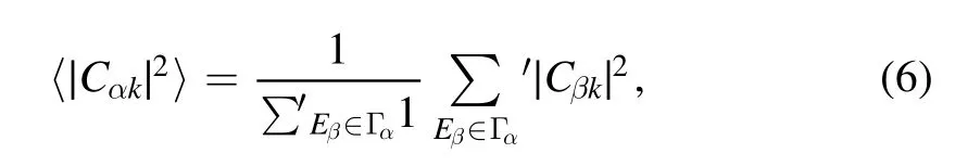
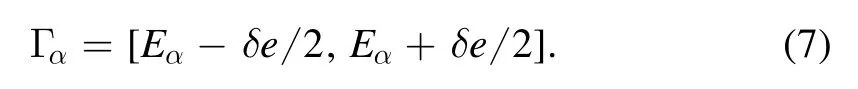
where Γαindicates a narrow energy window centered at Eαwith a small width δe,

In most physical models of realistic interest,there exist certain dynamic Lie groups behind them,such that observables of realistic interest are written as simple(at least not complicated)and regular functions of generators of the groups.In this paper,we study the distribution of rescaled componentsunder small perturbations of this type,to see whether it may supply information useful for the purpose of distinguishing between quantum chaotic and integrable systems.

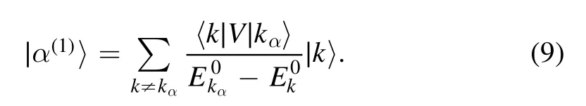
To achieve this goal,let us consider the first-order perturbation expansion of an arbitrary perturbed state|α〉.Using kαto indicate the label k for whichis the closest to Eα,under sufficiently weak perturbation,one writes

To analyze properties of the elementsVkkα,one may employ a basis,written as |n〉,which is given by states that are expressed as simple functions of generators of the underlying dynamic group.One may always find out an integrable Hamiltonian,denoted by Hint,which is a simple function of the generators and whose eigenstates are just the states |n〉.(For example,in some cases,Hintmay be the particle-number operators.)Generically,one writes

where U is an operator and λ is a running parameter,such that H0describes an integrable system at λ=0 and describes a chaotic system at λ lying within some large parameter regime.The eigenstates |n〉 of Hintwith energies ensatisfy

On the basis |n〉,the unperturbed states |k〉 are expanded as

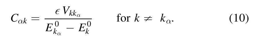
Let us first discuss an integrable Hamiltonian H0.In the case that H0is given by Hintwith λ=0,the states |k〉 are identical to the states |n〉.Since the operator V is a simple function of the above-discussed generators,by which the states|n〉are constructed,the matrix elementswhich are given by Vmn=〈m|V|n〉,are regular functions of the labels m and n.In fact,in most realistic models,these elements vanish for most pairs(m,n)in a Hilbert space not small.Then,from equation(10),one sees that the distribution of the rescaled componentsshould show notable deviation from the normal(Gaussian)distribution; in particular,in most realistic models,one may expect a high peak at the origin point of.

In the case that H0is integrable but not identical to Hint,if the components 〈n|k〉 are not quite complicated functions of the label n,it is straightforward to generalize discussions given above.One still reaches the conclusion of notable deviation of the distribution offrom the Gaussian distribution.

Next,we discuss a generic quantum chaotic system H0.As shown in[24],those components Dknof |n〉 whose corresponding tori lie in classically-energetically-allowed regions can be written in the following form

where 〈|Dkn|2〉 indicates the averaged shape of the EFs Dkn,defined in a way similar to that in equation(6),and Rknare random numbers with a Gaussian distribution.Clearly,the elements 〈k|V|kα〉 can be written in the following form,

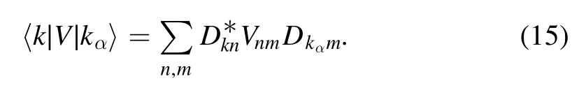
Usually,main bodies of the EFs of|k〉on the basis of|n〉lie in the corresponding classically-energetically-allowed regions.This implies that the expression in equation(14)should be valid for most significant components Dkn.Then,from equations(14)–(15),it is seen thatVkkαhave nonnegligible values with random signs for those states|k〉whose energiesare not quite far fromThis suggests that the distribution of the rescaled componentsfornot very far from Eαshould have a Gaussian form.

Numerical simulations

For the purpose of numerically testing the analytical predictions given above,we have employed a three-orbital Lipkin–Meshkov–Glick model[25].This model is composed of Ω particles,occupying three energy levels labeled by r=0,1,2,each with Ω-degeneracy.Here,we are interested in the collective motion of this model,for which the dimension of the Hilbert space isWe use ηrto denote the energy of the rth level and,for brevity,set η0=0.The Hamiltonian H0in equation(11)is given by[26]

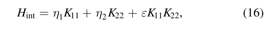
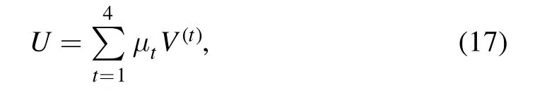
where ε and μtare parameters and

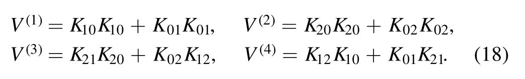
Here,Krrrepresent particle-number operators for the levels r and Krsof r≠s are particle raising and lowering operators,defined by

In our numerical simulations,we set V=U.Parameters fixed in our simulations are μ1=0.0032,μ2=0.0036,μ3=0.0039,μ4=0.0048,ε=10?6,and ?=10?3.The particle number is set at Ω=140,for which the dimension of the Hilbert space is dH=10011.The width δe is adjusted,such that each window Γαincludes 12 levels.In the computation of the distribution of components for a given pair of perturbed and unperturbed Hamiltonians,400 perturbed states|α〉 that lie in the middle energy region were used and,for each state |α〉,400 componentsof |k〉 in the middle energy region were used.

Let us first discuss the integrable case with λ=0 for H0.We took η1=0.3532 and η2=0.5714,for which the winding number is close to the golden meanThe distribution g(C)was found quite different from the Gaussian form,with a high peak in the middle region(figure 1),in agreement with the analytical predictions discussed above.

Next,we discuss quantum chaotic systems H0,whose nearest-level-spacing distribution is close to that predicted by the random matrix theory.In agreement with the analytical predictions,we found that the distribution g(C)is quite close to the Gaussian form.One example is given in figure 2 with λ=0.8.

We have further studied the process of transition of H0from integrable to chaotic.To be quantitative,we have computed the difference between the distribution of rescaled componentsand the Gaussian distribution,denoted by ΔEF

where gG(C)indicates the Gaussian distribution,

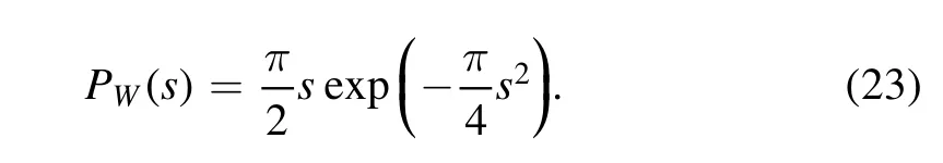
For comparison,we have also computed the following difference between the nearest-level-spacing distribution,denoted by P(s),and the Wigner distribution PW(s),that is

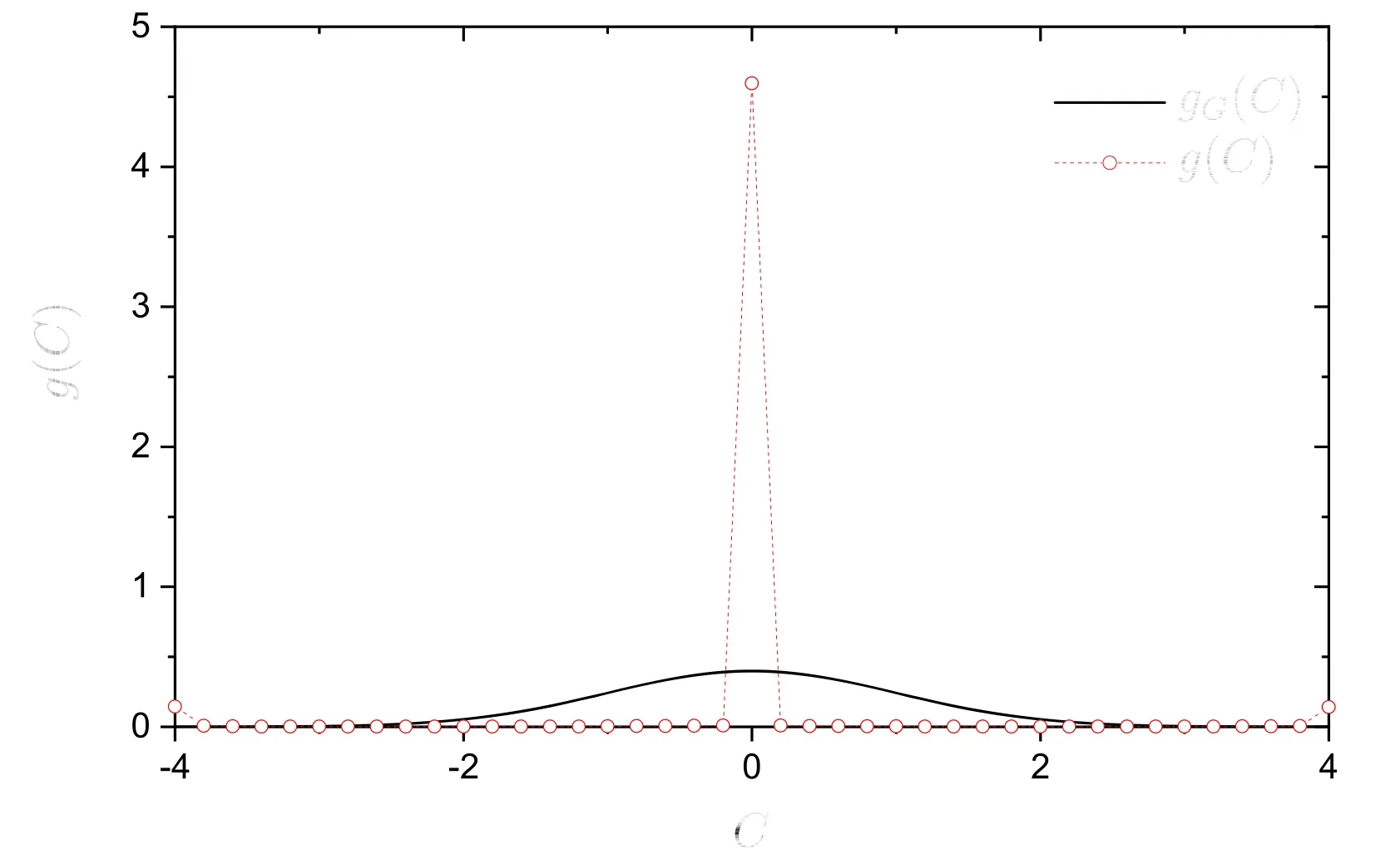
Figure 1.The distribution g(C)of rescaled EF components (circles connected with dotted line),for an integrable Hamiltonian H0 with λ=0,?=0.001,η1=0.3532,and η2=0.5714.The solid curve indicates the Gaussian distribution gG(C)in equation(21).

Figure 2.Similar to figure 1,but for a quantum chaotic system H0 with λ=0.8.

where

Variation of ΔEFand ΔEwith the parameter λ are shown in figure 3.It is seen that ΔEFchanges a little for λ up to 0.1,indicating that(0,0.1)should be a nearly integrable region of λ; it becomes quite small at λ>0.6.Qualitatively,these features are in consistency with features exhibited in ΔE.

Summary

In this paper,a method is proposed and used to show qualitative difference between EFs of integrable and chaotic quantum systems.The method is based on difference in the response of EFs to small perturbations.That is,for quantum chaotic systems,the response shows a random feature such that the distribution of rescaled components of the perturbed system is close to a Gaussian form.While,for quantum integrable systems,the distribution is far from the Gaussian form.This difference in the response is useful in the study of integrability-chaos transition of quantum systems and may be used as an indicator of quantum chaos.

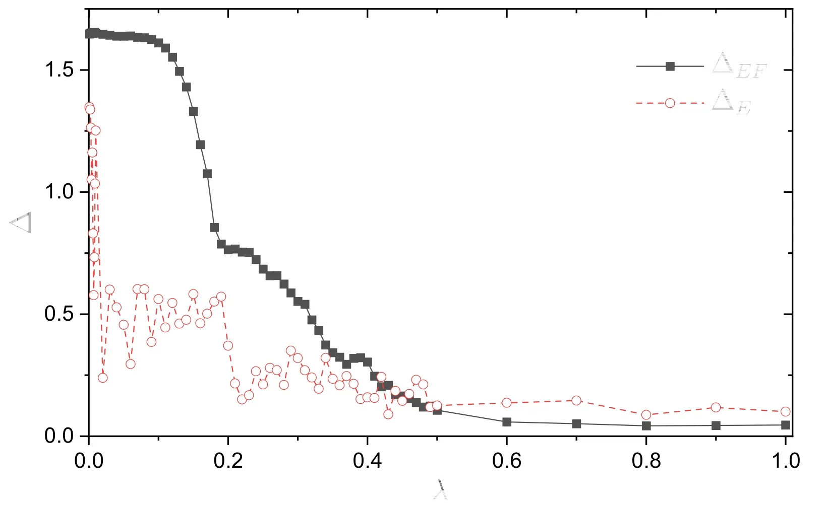
Figure 3.Variation of the deviation ΔEF(solid squares connected by solid line)and ΔE(open circles connected by dashed line)with the parameter λ.

Acknowledgments

This paper was supported by the National Natural Science Foundation of China under Grant Nos.11535011 and 11775210.