Zhi-Xuan Yang(楊智璇), Yi-Meng Zhang(張一萌), Yu-Xuan Zhou(周宇軒), Li-Bo Zhang(張禮博),Fei Yan(燕飛), Song Liu(劉松), Yuan Xu(徐源), and Jian Li(李劍),?

1Shenzhen Institute for Quantum Science and Engineering,Southern University of Science and Technology,Shenzhen 518055,China

2Guangdong Provincial Key Laboratory of Quantum Science and Engineering,Southern University of Science and Technology,Shenzhen 518055,China

3Shenzhen Key Laboratory of Quantum Science and Engineering,Southern University of Science and Technology,Shenzhen 518055,China

4Department of Physics,Southern University of Science and Technology,Shenzhen 518055,China

Keywords: superconducting qubit,circuit QED,Landau–Zener–St¨uckelberg interference

1. Introduction

Landau–Zener–St¨uckelberg (LZS) interference is a phenomenon that appears in a two-level quantum system undergoing periodic transitions between energy levels at the anticross.[1]Since the pioneering theoretical work by Landau,[2,3]Zener,[4]St¨uckelberg,[5]and Majorana[6]in 1932, profound explorations on LZS interference and related problems have been carried out both theoretically and experimentally in the past 90 years. In the 21st century, LZS interference and related research have become active again, owing to the enormous progress in experimental technologies for creating and manipulating coherent quantum states in solid-state systems.LZS interference patterns have been observed in the electronic spin of a double quantum dot,[7]charge oscillations of a double quantum dot,[8]electronic spin of nitrogen-vacancy(NV)center in a diamond,[9]and superconducting qubits.[10–13]Recently, a method using light propagating along the curved waveguides to simulate the time domain Landau–Zener transitions and LZS interferences has been proposed;[14]even in a hybrid system formed by a superconducting qubit coupled to an acoustic resonator,LZS interference has been studied.[15]

Unlike in double quantum dots and NV centers, natural microscopic particles such as electrons and atoms being used to perform experiments, superconducting qubits[16,17]consisting of Josephson junctions, inductors, and capacitors are true artificial macroscopic quantum objects. The macroscopic nature of superconducting qubits makes them not only an ideal testbed for quantum physics but also an advanced platform for emerging quantum information processing.[18]In the early stage of LZS interference experiments in superconducting qubits,[10–13]flux qubit,[19]charge qubit,[20]and phase qubit[21]have been used. These qubits have a fairly short coherence time of only a few nanoseconds,which makes observation of LZS dynamics,particularly the global structures[22](also called the Rabi-like oscillations[9,23]),which strongly depends on the initial phase of periodic transitions hardly possible.

A new type of charge-noise-insensitive superconducting qubit called transmon was invented in 2007.[24]By combining transmon with superconducting coplanar waveguide (CPW)resonator, a superconducting quantum circuit working in microwave regime and equivalent to optical cavity quantum electrodynamics (QED) can be formed, which is known as circuit QED.[25]In a circuit QED, the CPW resonator can protect the qubit from spontaneous decay and provide a highvisibility readout of qubit states. Owing to refinements in circuit design, material platform, and fabrication techniques in the past decade, circuit QED with transmon and its descendent Xmon[26]becomes the mainstream of superconducting quantum information processing.[27]Nowadays,the coherence time of a transmon or Xmon in a circuit QED system can easily be over 10μs,making it an excellent system for studying LZS dynamics.

In this paper, we adopt a circuit QED system consisting of an Xmon qubit, a transverse (XY) control line, a longitudinal (Z) control line, and a readout resonator to investigate LZS interference phenomena. By combining good coherence of the Xmon qubit and controlling the initial phase of periodic transitions,we demonstrate phase sensitivity of the qubit population in both time evolutions and steady states,and observe the Rabi-like oscillation for the first time in a superconducting quantum circuit. Since in our work the LZS interference does not happen in the Schr¨odinger picture,one may consider our system as a quantum simulator to mimic LZS physics in a rotating frame.

2. Physical model

The equivalent diagram of the circuit QED system is shown in the dashed box of Fig.1. The dual-junction Xmon qubit can be excited by a near-resonance microwave driving field sending to the XY control line. The qubit transition frequency can be tuned by magnetic flux threading the loop formed by the two Josephson junctions(the so-called dc SQUID),and the magnetic flux is controlled by sending a current to the Z control line. This tunability of qubit transition frequency gives rise to the periodic transitions required by the LZS process.

For an Xmon qubit, the flux dependent transition frequency is approximately

Here Φ is the flux threading Xmon’s dc SQUID loop, Φ0=h/(2e) is the magnetic flux quantum, ECand EJrepresent the single-electron charging energy and the total Josephson energy, respectively. From Eq. (1), one can easily find out that the qubit transition frequency is not linearly dependent on flux. Only when Φ/Φ0is far away from κ/2 (here κ is an arbitrary integer), ω10is near linearly dependent on Φ. If the total flux Φ consists of a dc part and an ac part Φ =Φdc+Φaccos(ωt+φ), and(Φdc±Φac)/Φ0is far away from κπ/2 (we may call the region far away from κπ/2 the near-linear region), the qubit transition frequency then becomes

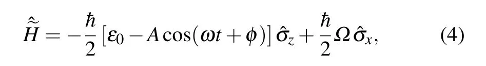
The Hamiltonian of an Xmon qubit flux biased in nearlinear region, with XY microwave drive, can then be written as

with XY drive frequency ωd, and Rabi frequency ?. For XY drive, a fixed phase 0 is assumed, so φ represents both the initial phase of periodic transitions(Z modulation)and the relative phase between Z modulation and XY drive.

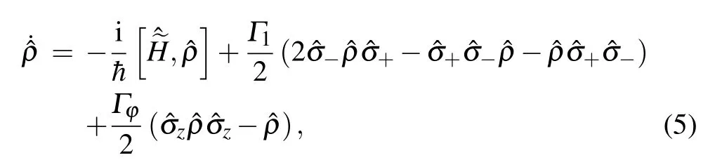
where ε0=ω0?ωdis the detuning between qubit transition and XY drive. This rotating-frame Hamiltonian is very similar to LZS models being studied in literatures such as Refs.[1,22].Taking relaxation and dephasing into account, time evolution of this system can be calculated by solving the Markov master equation[28]

3. Experimental setup

In previous experiments like Refs. [23,29,30], continuous microwaves were used for Z modulation and XY drive(if needed). By using continuous microwaves, only the steadystate properties of the systems can be studied. Since the relative phase φ is not locked during continuous-wave measurements, the steady states are averaged over φ; therefore, any phase-sensitive phenomenon is washed away by this phase averaging.

In order to obtain phase-sensitive evolutions, we need to control the relative phase φ precisely. In our experiments,we use pulsed Z modulation and standard IQ mixing technique for XY drive pulses to achieve phase control. As shown in Fig.1, the qubit XY drive is formed by mixing a continuous local oscillator (LO) microwave field (XYLO), with two pulsed quadratures(I and Q)generated by two channels of an arbitrary waveform generator (AWG), ωd=ωLO+ωIQ. The pulsed Z modulation signal is directly generated by another channel of the AWG.Since all channels of the AWG are synchronized,control φ is controlling the relative phase between signals from different channels. The Z modulation signal and a dc current for dc flux bias are combined by a bias-tee and sent to the Z control line of the Xmon.

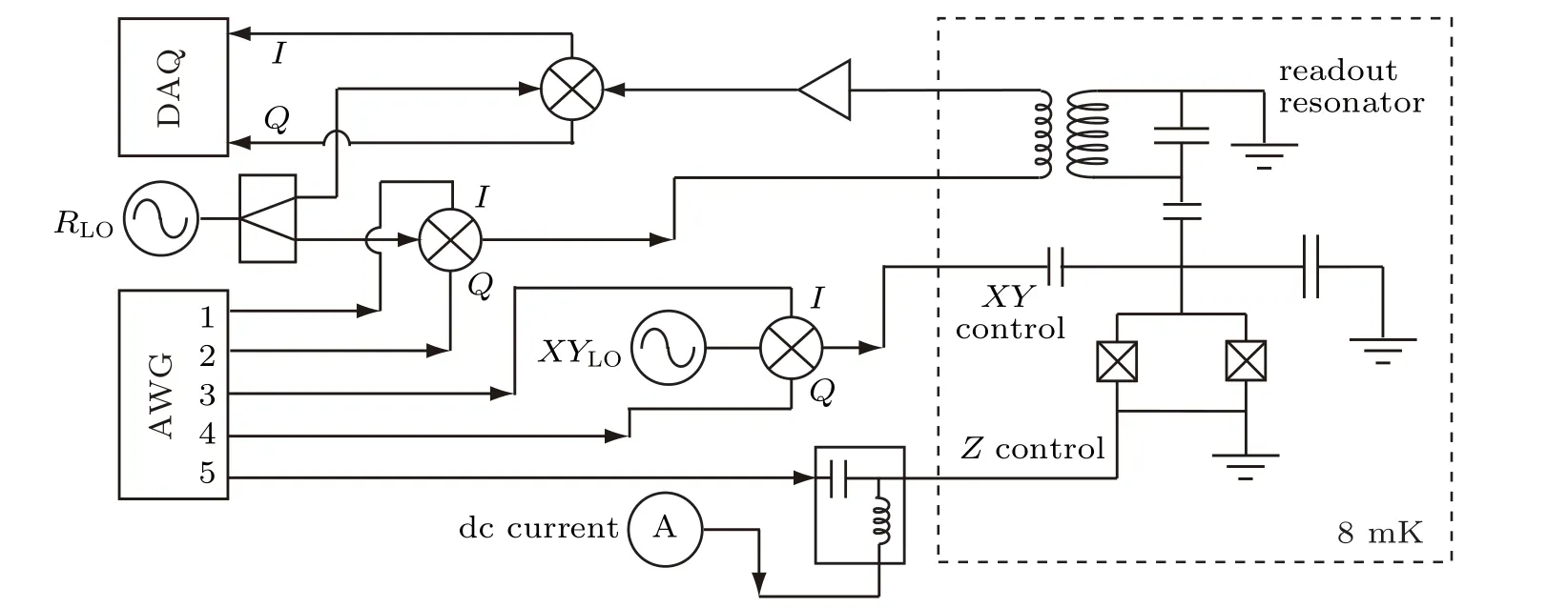
Fig.1. The schematics of the experimental setup. The circuit QED sample consisting of an Xmon qubit with XY, Z control lines, and a readout resonator is mounted to the mixing chamber (illustrated by the dashed box) of a dilution refrigerator. The room temperature equipment and components are shown on the left-hand side of this figure.

The qubit dispersive readout[31]pulses are generated in the same way as for XY drive pulses. The readout(R)pulses through the readout resonator, are amplified at both low temperature and room temperature, then are down-mixed (a reverse process of IQ mixing) and digitized by a data acquisition(DAQ)card. An illustration of pulse sequences is shown in Fig.2. One should note that,due to different cable lengths as well as different components on cables,even though pulses are generated by the AWG at the same time, there are constant delays between Z,XY,and R pulses when they reach the circuit QED sample at mixing chamber of the dilution refrigerator. To compensate for these delays,we let the Z modulation pulse a few tens of nanoseconds longer than the XY IQ pulses.

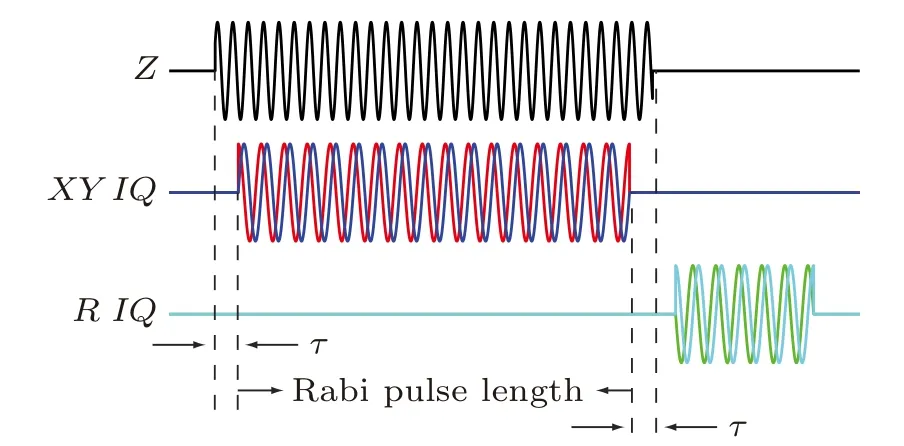
Fig.2. Schematic pulse sequences of one measurement cycle. Z modulation pulse is a simple cosine function cos(ωt+φ),and it is 2τ longer than XY IQ pulses,cos(ωIQt)and sin(ωIQt)define the Rabi pulse length and amplitude.

4. Results

4.1. Adiabatic limit

We first study the phase-dependent time evolution of qubit excited state (|1〉) population P|1〉in the adiabatic limit.?/2π=26.2 MHz,ω/2π=1.44 MHz,A/2π=72 MHz,and ε0=0 are taken. These values are close to those listed under Fig.3 of Ref.[22]. The relative phase φ is swept from 85?to 175?,and the measured results are shown in Fig.3(a). Numerical results by solving the master equation Eq. (5) are shown in Fig.3(b). One may find that φ in numerical simulation is from 0.2π to 0.7π. This is due to the delay between Z and XY pulses, as discussed in Section 3. To avoid confusing the experimental and numerical values of φ, we use numerical φ(in π)for the following discussions.

From both experimental and numerical results, we can find that the population evolution around φ = 0.5π differs from other φ values drastically. In Figs. 3(c) and 3(d), we plot the population evolution for φ =0.2π and φ =0.5π, respectively. Both experimental(black solid curves)and numerical(red dotted curves)results match Garraway and Vitanov’s prediction[22]well.

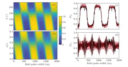
Fig.3. Evolution of P|1〉, with A/ω =50 and ?/ω =18.2. (a) Experimental data for different relative phase φ. (b) Numerical results corresponding to(a). (c)and(d)are P|1〉 time evolutions for φ =85?(0.2π)and φ =139?(0.5π),respectively. The black solid curves are experimental data,and the red dotted curves are numerical results.

4.2. The boundary between adiabatic and non-adiabatic limits

We then study the phase-dependent time evolution of P|1〉at the boundary between adiabatic and non-adiabatic limits,?2≈Aω. ?/2π = 12 MHz, ω/2π = 2.4 MHz, A/2π =63.75 MHz, and ε0= 0 are taken. The measured results and the corresponding numerical calculation results are shown in Figs. 4(a) and 4(b), respectively. Similar to the adiabatic limit, one can also find that the population evolution around φ =0.5π differs from other φ values drastically. A longer trace of P|1〉evolution at φ =0.5π is recorded, as indicated by the black solid curve in Fig.4(c). In this longer evolution trace, a Rabi-like oscillation is observed, with an oscillation frequency ?0much lower than any of ?, A,and ω. The numerical results for φ =0.5π trace are shown in Fig.4(d)as the red solid curve.

In Ref.[23],a formula for Rabi-like oscillation frequency

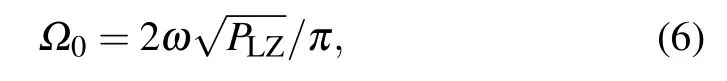
was derived, where PLZ=exp(?2πδ) is the Landau–Zener probability, and δ = ?2/(4Aω) as mentioned before. By putting the experimental values of ?, A, and ω into this formula, we get ?0≈2π×730 kHz, which differs from the fitting (the green dashed curves in Fig.4) value ?0=2π×390 kHz by roughly a factor of 2. Another formula

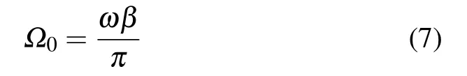
can be found in Eq.(28)of Ref.[22],with

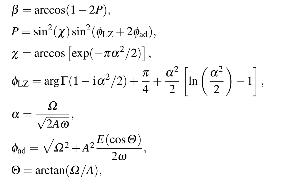
where Γ is the gamma function, and E is the complete elliptic integral of the second kind. Using this formula, we get?0≈2π×296 kHz,which also differs from the fitting value by about 100 kHz. We are not clear where these differences come from.

4.3. Phase-sensitive steady states

To study the phase-dependent steady-state population(LZS spectra), we take ?/2π =12 MHz, ω/2π =6 MHz,and sweep the Z pulse voltage from 3 mVppto 36 mVppwhich covers the adiabatic limit and the crossover to non-adiabatic limit. 40 μs long Rabi pulses are applied to ensure that the qubit is driven to a steady state, and the detuning ε0/2π is swept from ?40 MHz to 40 MHz. Figures 5(a)and 5(c)show the experimental data and the numerical calculation results for φ =0.4π,respectively.A weak asymmetry can be observed in LZS spectra.By increasing φ to 0.9π,the asymmetry becomes more visible,as indicated by Figs.5(b)and 5(d).

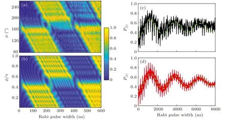
Fig.4. Evolution of P|1〉, with A/ω =26.6 and ?/ω =5. (a) Experimental data for different relative phase φ. (b) Numerical results corresponding to(a). (c)and(d)are experimental and numerical P|1〉 time evolutions for φ =176?(0.5π),respectively. The green dashed curves in(c)and(d)are the same,indicating a Rabi-like oscillation of frequency ?0=2π×390 kHz.

Fig.5. Steady-state P|1〉in adiabatic limit. (a)and(b)are experimental data for relative phases φ =44?and φ =134?,respectively. (c)and(d)are numerical results for φ =0.4π and φ =0.9π,respectively.

5. Conclusion

We have experimentally and numerically explored the phase-sensitive LZS phenomena using a superconducting Xmon qubit. By choosing such a dc flux bias point, to let the qubit transition frequency near-linearly respond to ac flux modulation,and to let the qubit have a proper dephasing time,we have not only studied the time evolution of the qubit population,but also for the first time observed phase dependence in steady-state population. A LZS induced Rabi-like oscillation is observed at the boundary between adiabatic and nonadiabatic limits. Though in this work,not much attention has been paid to the LZS process in the non-adiabatic limit, superconducting Xmon qubit and IQ mixing technique indeed provide a powerful platform for investigating LZS problems in all parameter regimes.

Appendix A:Flux modulation of an Xmon qubit

For simplicity,we suppose the two Josephson junctions of the Xmon are identical and limit the flux ?0.5 ＜Φ/Φ0＜0.5.The Hamiltonian of the Xmon reads

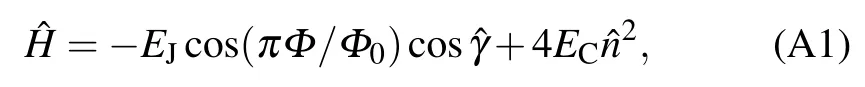
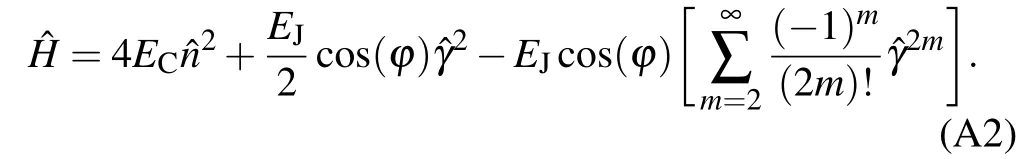
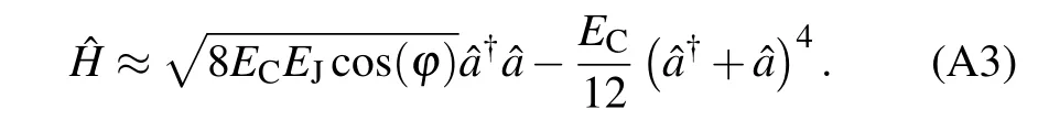
The first two terms on the right-hand side of Eq.(A2)form a simple harmonic oscillator(SHO).Then expressed in terms of SHO creation and annihilation operators, this Hamiltonian is approximately

Now we consider that the flux consists of dc and ac parts,? =?dc+?ac(t), and expand cos(?) to the leading order of ?ac(t),

we can rewrite the Hamiltonian as

Assuming the ac flux has the form ?ac(t)=?accos(ωt+φ),and truncating the Hamiltonian Eq.(A7)to its lowest two energy levels,we get

with ω0=ωp?EC/ˉh,and A=ωp?actan(?dc)/2.

Appendix B:Calibrations of parameters

Figure B1 shows the Xmon spectra with only dc flux bias.Due to the relatively strong XY drive amplitude used in spectroscopy, the two-photon transition process coupling Xmon’s ground state |0〉 and second excited state |2〉 is observed (the less visible parallel curve under the main spectra curve). The frequency difference(132 MHz for this sample)between this two-photon transition and the single-photon|0〉to|1〉(Xmon’s first excited state)transition is approximately EC/(2h)[24].By fitting the|0〉to|1〉transition(qubit)frequencies with Eq.(1),as shown by the white dashed curve in Fig.B1,we obtain the Josephson energy of this Xmon EJ=h×13.822 GHz.

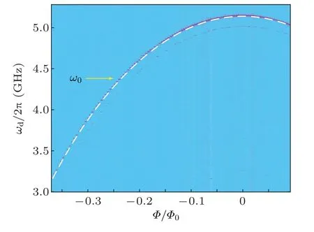
Fig.B1. Qubit transition frequency versus flux. The |0〉→|1〉 transition frequencies are fitted (the white dashed curve) by EC/h=0.264 GHz and EJ/h=13.822 GHz.

Figure B2(a) shows the calibration of Rabi frequency? for different XY IQ pulses peak-to-peak voltages at qubit frequency 4.365 GHz. The Z modulation frequency ω is precisely known in experiments, but the modulation amplitude A of qubit transition frequency can not be directly measured.In the small coupling regime ? ?ω,the qubit|1〉state population is approximately zero if the n-th Bessel function of the first kind Jn(A/ω)equals zero. Therefore the modulation amplitude A for different Z pulse peak-to-peak voltage can be calibrated using, e.g., the first zero of J0(A/ω), at which A ≈2.4ω. To do this calibration,we set detuning ε0=0 and Rabi frequency ?/2π = 2.5 MHz, then find Z pulse peakto-peak voltages corresponding to zero population for various modulation frequencies ω/2π =10,15,20,25,30 MHz. The calibration result is shown in Fig.B2(b).

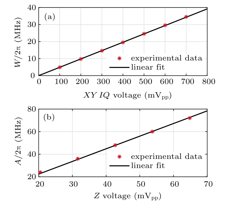
Fig.B2. Calibrations of(a)Rabi frequency ? versus XY IQ pulses peak-topeak voltage,and(b)Z modulation amplitude A versus Z pulse peak-to-peak voltage.

Acknowledgment

Enlightening and fruitful discussions with Professor Barry Garraway at the University of Sussex is gratefully acknowledged.