Xiaoyong Qian(錢驍勇), Dianchen Lu(盧殿臣), Muhammad Arshad,?, and Khurrem Shehzad

1Faculty of Science,Jiangsu University,Zhenjiang 212013,China

2Department of Mathematics and Statistics,University of Agriculture Faisalabad,Pakistan

Keywords: extended F-expansion method, generalized exp(?φ(ξ))-expansion technique, perturbed Kaup–Newell Schr¨odinger equation,traveling wave solutions

1. Introduction

Analytical wave results in dissimilar kinds play an important role in realization of nonlinear physical and mathematical phenomena in the fields of hydrodynamics, plasma physics,nonlinear optics, elastic media, problems of biological, engineering and optical fibers.[1–12]The fascinating technology of sub-pico second pulses that propagate through optical fibers is modeled with the Kaup–Newell equation. Several decades ago,this famous model was first proposed by David Kaup and Alen Newell, and is one of the three forms of the derivative nonlinear Schr¨odinger equation(NLSE)that governs the soliton dynamics.The research of soliton solutions has been of appreciable significance for knowing nonlinear phenomena over the recent years. To know the integrability nature in ordinary and partial differential equations,[1,2]the theory of solitons has enhanced in recent decades. The derivative NLSE is

It is also named as the Kaup–Newell (K–N) model,[3]which has several sensual applications, particularly in nonlinear optics and plasma physics. In several models, the derivative nonlinear Schr¨odinger equation (DNLSE) was studied to exhibit the molecule of soliton propagation throughout an optical fiber. The DNLSE has many forms which are identified,such as the Gerdjikov–Ivanov equation(GIE),the Chen–Lee–Liu equation (CLLE), and the K–N equation. Alternatively, these equations are named as DNLSE-I, DNLSE-II and DNLSE-III. Through the Gauge transformation,[9]these equations can be altered to each other. In scattering problems,the transformations cannot preserve the condition of reduction. However, the transformations cannot conserve the condition of reduction in the scattering model and extremely intricate integral is involved, and it cannot be premeditated explicitly.[10,11,13]Therefore,they merit to be investigated independently. There is an abundance of mathematical techniques that are found to tackle these assortment of nonlinear Schr¨odinger problems.[8,12,14–21]Recently, the perturbed Kaup–Newell(K–N)model[22,23]is introduced from the generalized Kaup–Newell spectral equation with linear perturbations as follows:

where the function u(x,t)indicates the wave function of complex valued. The variables x and t represent the spatial and temporal coordinates, respectively. The first term on the lefthand side of Eq.(2)indicates the temporal evaluation,and the second term indicates the group velocity dispersion having coefficient α1. The third term together with coefficient α2provides nonlinear effect. On the right-hand side of Eq.(2),coefficient β indicates inter-model dispersion,η and δ indicate the self-steepening and nonlinear dispersion effects. Lastly, the parameter for full nonlinearity is m.To date,researchers[22–25]have been successfully shown the mathematical engineering of Eq.(2).

This article will study the exact solution of the K–N equation with some hamiltonian sort perturbation terms. Fexpansion and exp(?φ(ξ))-expansion schemes executed to construct soliton solution to the current K–N equation. The achieved solutions are novel. The stability of achieved solutions are also examined via utilizing modulation instability(MI)analysis. After brief introduction,the K–N equation details are given in the rest of the paper.

2. Depiction of proposed techniques

In this section, we elucidate the algorithm of projected methods, namely, the modified F-expantion method and the generalized exp(?φ(ξ))-expantion technique for finding the exact solutions of the K–N model. A general non-linear evolution equation has the form of

where the function w(x,t)is unknown,and polynomial Q has some specified functions or variables,which also contains both linear and non-linear derivative terms of the w(x,t). Considering the transformation for switching independent variables into one variable yields

where k and ν are wave length and frequency. Utilizing Eq. (4), equation (3) is diminished into the ordinary differential equation

where ψ′= dψ/dξ.

2.1. Modified F-expantion method

The major stages of this scheme are stated in the following.

First stepConsider the solution to ODE(5)has the form of

where the constants aiand n are real.F(ξ)ensures the following new ansatz equation:

where d0,d1,d2and d3are real constants.

Second stepN is a positive integer and it is generally found via utilizing homogeneous balance principle on Eq.(5),and the coefficients series a?N,a?N+1,...,a0,a1,...,aN,ν,k,n are obtained.

Fourth stepThe solutions to Eq.(5)can be achieved by deputing the values achieving in the third step into Eq.(6).

2.2. Generalized exp(?φ(ξ))-expansion technique

The major stages of this scheme are given in the following.

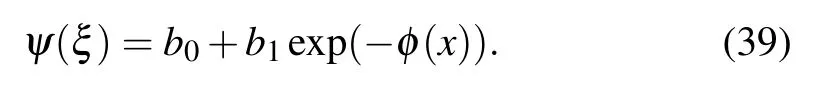
First stepConsider the solution to ODE(5)has the form of

where bi(0 ≤i ≤N)represents constants we have to calculate, such that bN/=0 and φ =φ(ξ) satisfies the following auxiliary ODE:

where r, p and q are constants.

Second stepPositive integer N can be calculated by using homogeneous balance principle between nonlinear terms occurring and derivative terms of highest order in Eq.(5).

Third stepSubstituting Eqs. (8) and (9) into Eq. (5)yields a polynomial in e(?φ(ξ)). Putting different powers of(e(?φ(ξ)))ito zero,we can reach algebraic equations. Solving this system and back substitutions, we attain a set verity of exact solutions to Eq.(3).

3. Application of proposed methods to the perturbed K–N Schro¨dinger equation

In this section, we construct the soliton solutions to the perturbed K–N equation by utilizing two mathematical techniques.

3.1. The modified F-expansion method

As Eq.(2)is complex,so our hypothesis of the wave solution to Eq.(2)is in the form of

where ψ(ξ) is given in Eq. (6); k, ν, γ, ω, and ε are arbitrary constants; ψ(ξ) is the amplitude component of the wave profiles; P is the phase factor; γ, ω, and ε show the frequency, wave number, and phase constant, respectively.Putting Eq. (10) into Eq. (2) and making separate into parts yield

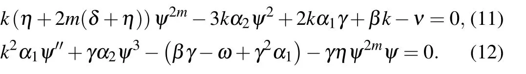
Substituting ψ2mfrom Eq.(11)into Eq.(12)yields

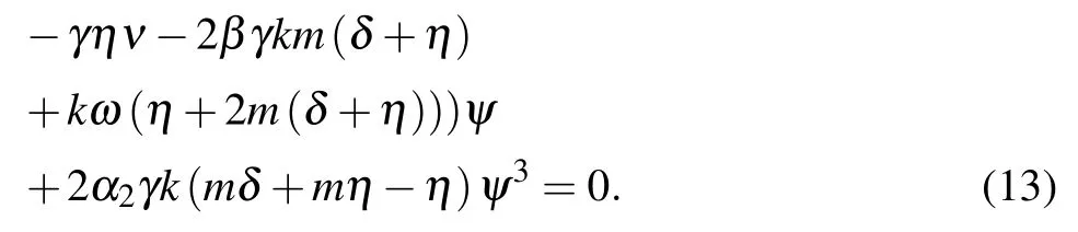
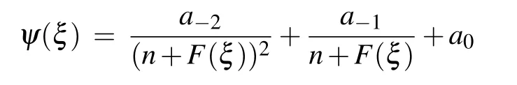
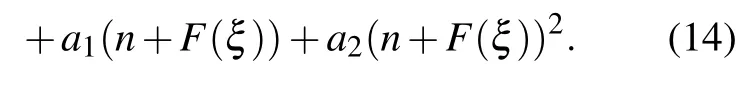
Apply balance principle of homogeneity on Eq.(13)and consider the solution to Eq.(13)to be

Family 1In this family,we consider d0=d3=0,

Set 1:

Set 2

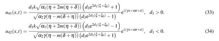
We can achieve the soliton solutions to Eq.(2)from set 1 in the form as follows:

We also achieve more soliton solutions to Eq.(2)from set 2 as

Family 2In this family,we consider d1=d3=0,

Set 1

Set 2

The wave solutions to Eq.(2)are achieved from solution set 1 as follows:

We attain more exact solutions to Eq.(2)from solution set 2 as

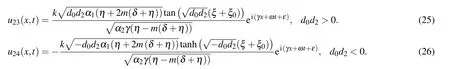
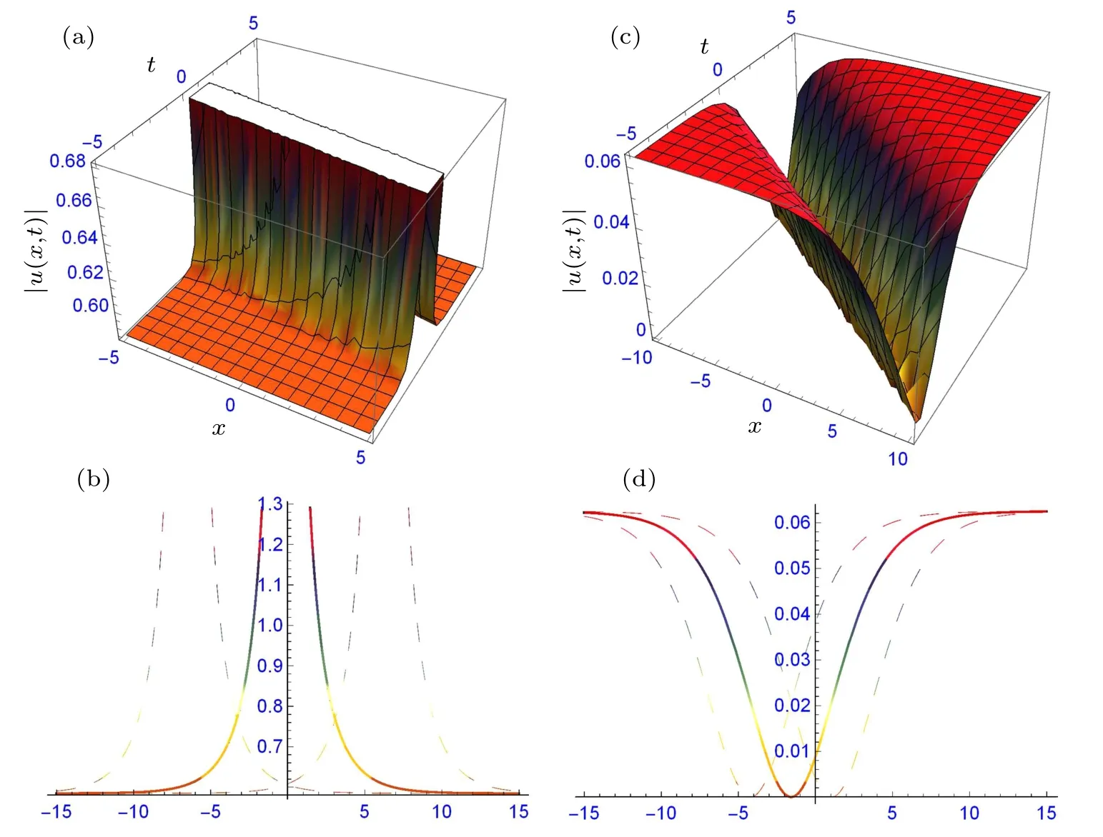
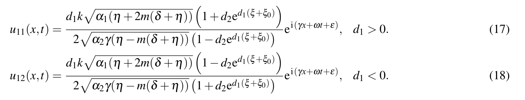
Fig.1. The structure of solutions (17) and (18): (a) bright solitary wave and its two-dimensional profile (b), and (c) dark soliton and its two-dimensional profile(d),providing suitable values to the parameters.

Family 3In this family,we consider d3=0,

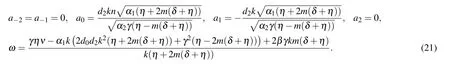
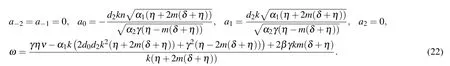
Set 1

Set 2

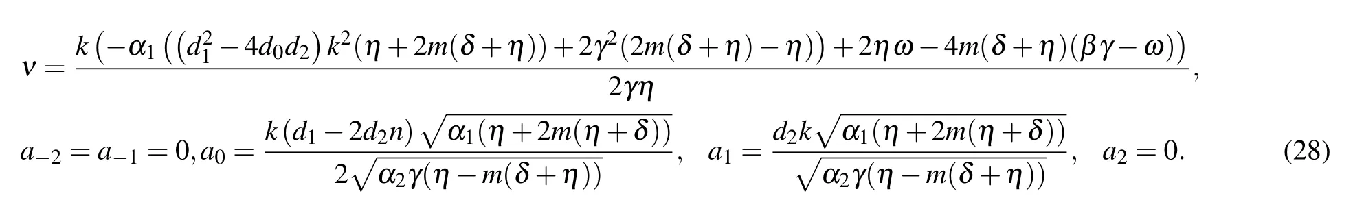
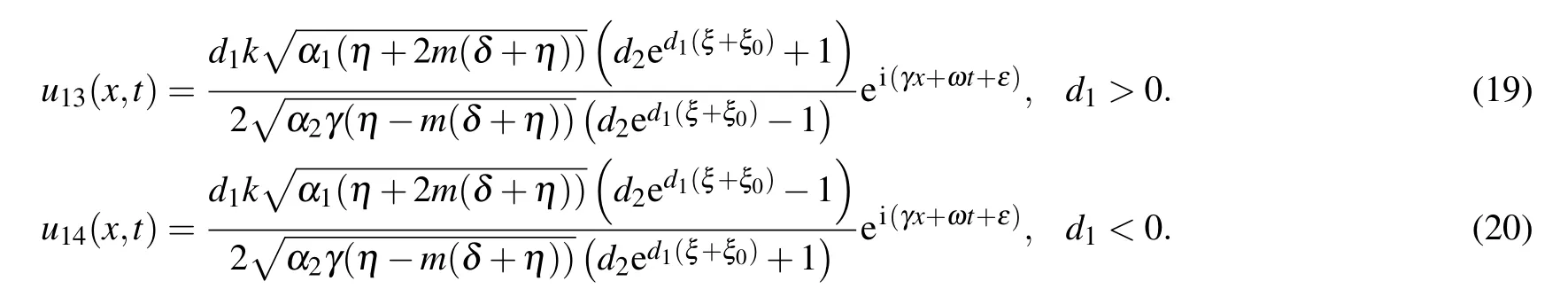
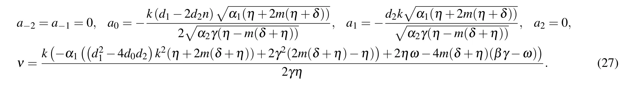
The wave solutions to Eq.(2)from sets 1 and 2 are constructed as follows:

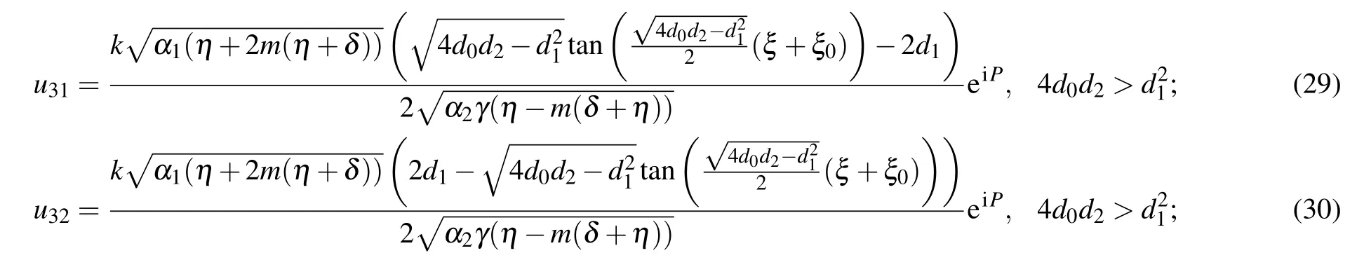
where ξ0is constant and P=γx+ωt+ε.

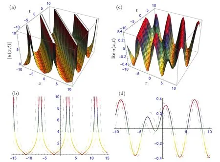
Fig.2. The structure of solutions(26)and(27): (a)periodic solitary waves and the two-dimensional profile(b),and(c)combined bright-dark solitary wave and its two-dimensional profile(d),providing suitable values to the parameters.

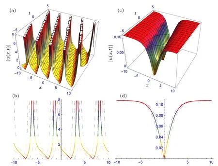
Fig.3. The structure of solutions (29) and (34): (a) periodic waves and the two-dimensional profile (b), and (c) dark soliton and its twodimensional profile(d),providing suitable values to the parameters.

Family 4In this family,we consider d0=d2=0,

Set 1

Set 2

The following soliton solutions to Eq.(2)from set 1 are attained as follows:

Similarly,one can construct more soliton solutions to Eq.(2)from set 2.

3.2. Generalized exp(?φ(ξ))-expansion technique

As Eq. (2) is complex, our hypothesis of the wave solution to Eq.(2)is in the form of

where ψ(ξ)is given in Eq.(8). Putting Eq.(35)into Eq.(2)and making separate into parts yield

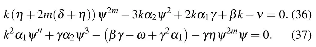
Substituting ψ2mfrom Eq.(36)into Eq.(37)yields

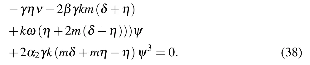
The homogeneous balance principle is applied on Eq. (38),and we consider the solution to Eq.(13)as follows:

Family 1

From family 1,the following kinds of soliton solutions to Eq.(2)are constructed.

Type IFor r=1, p/=0,q2?4p>0,

Type IIFor r=1, p/=0,q2?4p ＜0,

Type IIIFor r=1, p=0,q/=0,q2?4p>0,

Type IVFor r=1, p/=0,q/=0,q2?4p=0,

Type VFor q=0,r>0, p>0,

Type VIFor q=0,r ＜0, p ＜0,

Type VIIFor q=0,r>0, p ＜0,

Type VIIIFor q=0, r ＜0, p>0,

Type IXFor p=0, q=0,

Family 2

Similarly,one can construct more general soliton solutions to Eq.(2)from family 2.

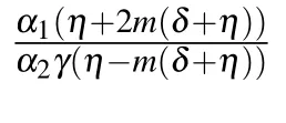
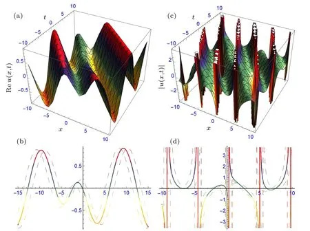
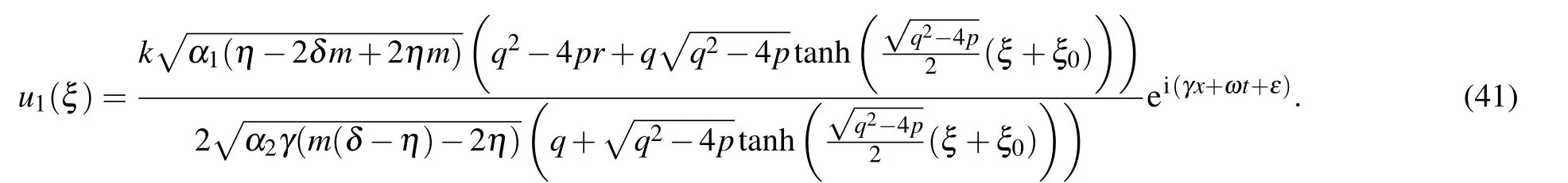
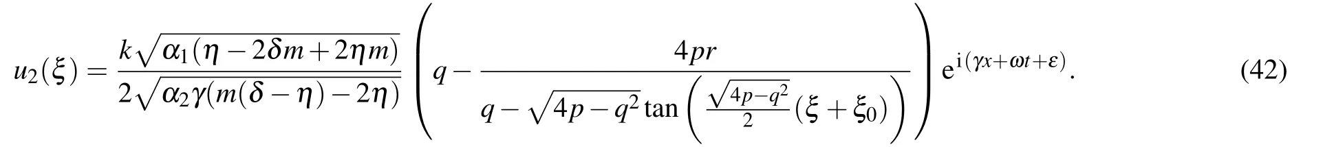
Fig.4. The structure of solutions (41) and (42): (a combined bright-dark solitary wave and its two-dimensional profile (b), and (c) periodic traveling wave and its two-dimensional profile(d),providing suitable values to the parameters.

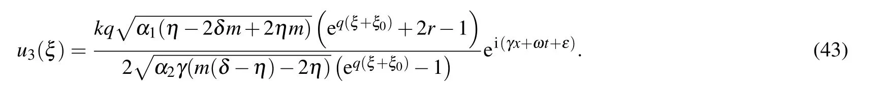
Fig.5. The structure of solutions(43)and(44): (a)bright-dark solitary wave and its two-dimensional profile(b),and(c)traveling wave and its two-dimensional profile(d),providing suitable values to the parameters.

4. Modulation instability

Numerous higher order nonlinear evolution equations depicting an instability that directs to investigate the steady state modulation as an consequence of the interaction among nonlinear and dispersive effects. To examine the MI of perturbed Kaup–Newell Schr¨oodinger Eq. (2) with using the analysis of standard linear stability[8,26–29]to scrutinize how weak and time dependent perturbations construct along the propagation distance. The steady state solution to the perturbed Kaup–Newell Schr¨oodinger equation reads

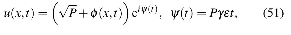
where P is normalized optical power. The perturbation φ(x,t)is studied by employing linear stability analysis. Substituting Eq.(51)into Eq.(2)and linearizing,we obtain

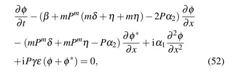
where ?denotes complex conjugate. Assume the solution to Eq.(52)as follows:

where k and τ are normalized wave number and frequency of φ(x,t). Substituting Eq.(53)into Eq.(52), we attain the dispersion relation(DR)

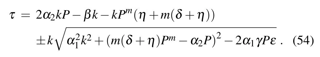
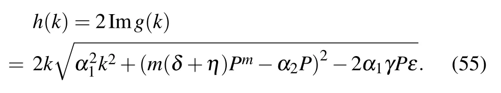
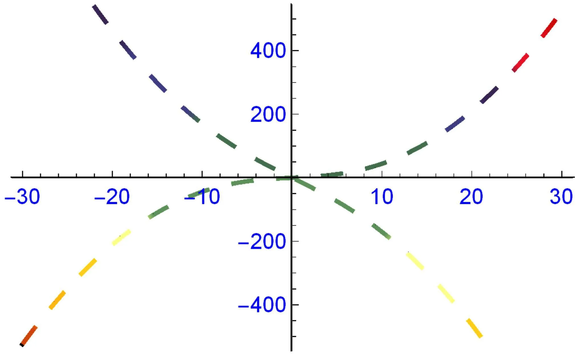
Fig.6. The graph of dispersion relation τ =τ(k).

5. Results and discussion

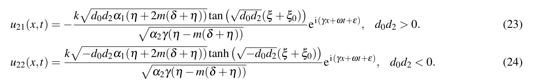
The achieved solutions are dissimilar from the attained results of numerous researchers by other prior techniques due to fact that the supposed result(14)of the proposed technique is changed from the previous technique. Equation (7) gives a few distinct type of solutions by providing dissimilar value of parameters. The authors of Ref. [23] constructed the solitons to Eq. (2) using the G′/G2-expansion and exp(??(ζ))-expansion methods. The obtained solutions (41), (42), (44),and(35)are similar to the solutions(23),(24),(26)and(27),respectively,which were obtained by authors of Ref.[23].The authors of Ref.[30]investigated the conservation laws of this dynamical model. Therefore, we have achieved several innovative results that have not been stated before.

Figures 1–3 signify the solitary waves in different shapes depicted. Figures 1(a)–1(d) depict the bright solitary wave and dark soliton in three and two-dimensional form of solutions (17) and (18) at α1=0.5, α2=1, β =0.25, γ =0.5,d1=0.5, d2=0.75, δ =1, η =0.5, k =1, m=1, n=1,ω = 1, ε = 1 and α1= 0.5, α2= 1, β = 0.25, γ = 0.5,d1=?0.5, d2=0.75, δ =1, η =0.5, k=1, m=1, n=1,ω =1, ε =1, respectively. Figures 2(a)–2(d) depict the periodic and combined bright-dark solitary waves in three- and two-dimensional forms of solutions(29)and(34)at α1=0.5,α2= 0.25, β = 0.4, γ = 0.5, d0= 0.5, d2= 1.5, δ = 1,η=0.25,k=0.5,ν=0.5,m=1,n=1,ξ0=1,ε=?1.5 and α1=0.5,α2=?1.3,β =?0.3,γ =1,d0=0.5,d2=?1.5,δ =?1.6,η=?0.05,ξ0=1,k=0.5,ν=0.5,m=1,n=1,ε =?0.5 respectively. Figures 3(a)–3(d) depict the periodic and dark solitary waves in three- and two-dimensional forms of solutions(29)and(34)at α1=0.5,α2=?1.3,β =?0.3,γ = 0.75, d0= 0.5, d1= 0.5, d2= ?1, δ = 1.6, η = 1,ξ0=?1,k=1,m=1,n=1,ω=0.5,ε=?0.5 and α1=0.5,α2=?1.3,β =?0.3,γ=0.75,d1=?0.5,d3=1,δ =?1.6,η =1, ξ0=0, k=1, m=1, n=1, ω =0.5, ε =?0.5, respectively.

Figures 4 and 5 describe the soliton and solitary waves in different forms depicted. Figures 4(a)–4(d)depict the combined bright-dark and periodic traveling waves in three- and two-dimensional forms of solutions(41)and(42)at β =0.5,p=0.5,q=1.5,r=1,α1=0.5,α2=?1.3,γ=0.5,ω=0.5,ε =?1.5, k =1, m=1, η =?0.05, ξ0=1 and β =0.5,p=1,q=1.5,r=1,α1=0.5,α2=?1.3,γ =0.5,ω =0.5,ε=?1.5,k=1,m=1,η=?0.05,ξ0=1,respectively. Figures 5(a)–5(d) depict the bright-dark and traveling waves in three-and two-dimensional forms of solutions(43)and(44)at β =0.5, p=0,q=1.5,r=1,α1=0.5,α2=?1.3,γ =0.5,ω =0.5, ε =?1.5, k =1, m=1, η =?0.05, ξ0=1 and β =0.5, p=1, q=2, r=1, α1=0.5, α2=?1.3, γ =0.5,ω =0.5,ε =?1.5,k=1,m=1,η =?0.05,ξ0=1,respectively. The dispersion relation τ =τ(k) between k and τ of perturbation is given in Fig.6.

6. Conclusion

We have employed the extended F-expansion and generalized exp(?φ(ξ))-expansion methods on the perturbed K–N equation, where the perturbation terms appear with full nonlinearity and traveling wave solutions in dissimilar forms such as bright and dark solitons, combined dark-bright solitons,solitary waves, periodic and other wave solutions attained.These obtained results are very helpful in governing soliton dynamics. This dynamical model describes plus propagation in optical fibers and can be observed as a special case of the generalized higher order NLSE.These achieved solutions are novel and may be useful for physicians, mathematician and engineers to understand more complex physical phenomena.These achieved soliton solutions have key applications such as optical fibers and ultra short light pulses.[5,31,32]The stability of model is discussed by utilizing modulation instability analysis, which confirms that all exact solutions are stable. The moments of a few results are revealed graphically by granting suitable values to parameters.In future to extend the result,we can solve the generalized higher order NLSE in the presence of non-local perturbation terms. The computation work endorses the simplicity,effectiveness and impact of current techniques.