Keju Tng, Xioling Wn*, Qifeng Lio

a School of Information Science and Technology, ShanghaiTech University, Shanghai 201210, China

b Department of Mathematics and Center for Computation and Technology, Louisiana State University, Baton Rouge, LA 70803, USA

Keywords:Deep learning Density estimation Optimal transport Uncertainty quantification

ABSTRACT In this work, we develop an invertible transport map, called KRnet, for density estimation by coupling the Knothe–Rosenblatt (KR) rearrangement and the flow-based generative model, which generalizes the real-valued non-volume preserving (real NVP) model (arX-iv:1605.08803v3). The triangular structure of the KR rearrangement breaks the symmetry of the real NVP in terms of the exchange of information between dimensions, which not only accelerates the training process but also improves the accuracy significantly. We have also introduced several new layers into the generative model to improve both robustness and effectiveness, including a reformulated affine coupling layer, a rotation layer and a component-wise nonlinear invertible layer. The KRnet can be used for both density estimation and sample generation especially when the dimensionality is relatively high. Numerical experiments have been presented to demonstrate the performance of KRnet.

Density estimation is a challenging problem for high-dimensional data [1]. Some techniques or models have recently been developed in the framework of deep learning under the term generative modeling. Generative models are usually with likelihood-based methods, such as the autoregressive models [2–5],variational autoencoders (VAE) [6], and flow-based generative models [7–9]. A particular case is the generative adversarial networks (GANs) [10], which requires finding a Nash equilibrium of a game. All generative models rely on the ability of deep nets for the nonlinear approximation of high-dimensional mapping.

We pay particular attention to the flow-based generative models for the following several reasons. First, it can be regarded as construction of a transport map instead of a probabilistic model such as the autoregressive model. Second, it does not enforce a dimension reduction step as what the VAE does. Third,it provides an explicit likelihood in contrast to the GAN. Furthermore, the flow-based generative model maintains explicitly the invertibility of the transport map, which cannot be achieved by numerical discretization of the Monge?Ampére flow [11]. In a nutshell, the flow-based generative model is the only model that defines a transport map with explicit invertibility. The potential of flow-based generative modeling is twofold. First, it works for both density generation and sample generation at the same time. This property may bring efficiency to many problems. For example, it can be coupled with the importance sampling technique [12] or used to approximate the a posterior distribution in Bayesian statistics as an alternative of Markov chain Monte Carlo (MCMC) [13]. Second, it can be combined with other techniques such as GAN or VAE to obtain a refined generative model[14, 15].

The goal of flow-based generative modeling is to seek an invertible mapping Z =f(Y)∈Rn, where f (·) is a bijection, and Y,Z ∈Rnare two random variables. Let pYand pZbe the probability density functions (PDFs) of Y and Z, respectively. We have

To construct f (·), the main difficulties are twofold: (1) f (·) is highly nonlinear since the prior distribution for Z must be simple enough, and (2) the mapping f (·) is a bijection. Flowbased generative models deal with these difficulties by stacking together a sequence of simple bijections, each of which is a shallow neural network, and the overall mapping is a deep net.Mathematically, the mapping f (·) can be written in a composite form:

where f[i]indicates a coupling layer at stage i . The mapping f[i](·)is expected to be simple enough such that its inverse and Jacobi matrix can be easily computed. One way to define f[i]is given by the real NVP [8]. Consider a partition y =(y1,y2) with y1∈Rmand y2∈Rn?m. A simple bijection f[i]is defined as

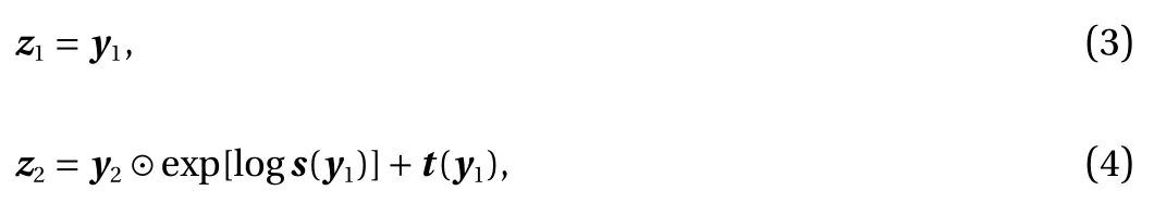
where s and t stand for scaling and translation depending only on y1, and ⊙ indicates the Hadamard product or componentwise product. When s (y1)=1, the algorithm becomes non-linear independent component estimation (NICE) [7]. Note that y2is updated linearly while the mappings s (y1) and t (y1) can be arbitrarily complicated, which are modeled as a neural network(NN),

The simple bijection given by Eqs. (3) and (4) is also referred to as an affine coupling layer [8]. The Jacobian matrix induced by one affine coupling layer is lower triangular:

whose determinant can be easily computed as

Since an affine coupling layer only modifies a portion of the components of y to some extent, a number of affine coupling layers need to be stacked together to form an evolution such that the desired distribution can be reached.

In the optimal transport theory, a mapping T :Z →Y is called a transport map such that T#μZ=μY, where T#μZis the push-forward of the law μZof Z such that μY(B)=μZ(T?1(B)) for every Borel set B [16]. It is seen that T =f?1, where f (·) is the invertible mapping for the flow-based generative model. In general, we have Yi=T(Z1,Z2,...,Zn) or Zi=f(Y1,Y2,...,Yn), i.e., each component of Y or Z depends on all components of the other random variable. The Knothe–Rosenblatt (KR) rearrangement says that the transport map T may have a lower-triangular structure such that

It is shown in Ref. [17] that such a mapping can be regarded as a limit of a sequence of optimal transport maps when the quadratic cost degenerates. More specifically, the Rosenblatt transformation is defined as

where

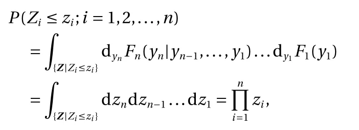
which implies that Ziare uniformly and independently distributed on [0 ,1]. Thus the Rosenblatt transformation provides a lower-triangular mapping to map Z , which is uniform on [0,1]nand has i.i.d. components, to an arbitrary random variable Y.

Motivated by the KR rearrangement, we propose a block-triangular invertible mapping as a generalization of real NVP. Consider a partition of y =(y1,y2,...,y∑K), where yi=(yi,1,yi,2,...,yi,m)with 1 ≤K ≤n and 1 ≤m ≤n , anddim(yi)=n. We define an invertible bijection, called KRnet,

whose structure is consistent with the KR rearrangement. The flow chart of KRnet is illustrated in Fig. 1. Before a detailed explanation of each layer, we fist look at the main structure of KRnet, which mainly consists of two loops: outer loop and inner loop, where the outer loop has K ?1 stages, corresponding to the K mappingsin Eq. (9), and the inner loop has L stages,corresponding to the number of affine coupling layers.

● Inner loop. The inner loop mainly consists of a sequence of general coupling layers, based on whichcan be written as:

where LRis a rotation layer and LSis a squeezing layer. The general coupling layerincludes a scale and bias layer,which plays a similar role to batch normalization.

For all general coupling layerswe usually let neural network Eq. (5) have two fully connected hidden layers of the same number of neurons, say l. Since the number of effective dimensions decreases as k increases in the outer loop, we expect that l decreases accordingly. We define a ratio r <1. Ifhas M hidden neurons in total, the number becomes M rk?1for.We now explain each layer in Fig. 1.

Squeezing layer.In the squeezing layer, we simply deactivate some dimensions using a mask

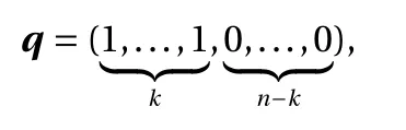
which means that only the first k components, i.e., q ⊙y, will be active after the squeezing layer while the other n ?k components will remain unchanged.

Rotation layer.We define an orthogonal matrix

where W ∈Rk×kwith k being the number of 1's in q, and I ∈R(n?k)×(n?k)is an identity matrix. Using, we obtainsubject to a rotation of the coordinate system. The Jacobian matrix betweenand y iswhose determinant is needed. For the sake of computation, we consider in reality:

where W =LU is the L U decomposition of W. More specifically,L is a lower-triangular matrix, whose entries on the diagonal line are 1, and U is a upper-triangular matrix. Then we have

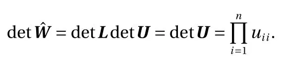
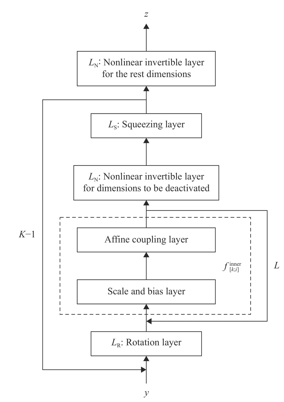
Fig. 1. Flow chart of KRnet

One simple choice to initializeis, where the column vectors of V are the eigenvectors of the covariance matrix of the input vector. The eigenvectors are ordered such that the associated eigenvalues decrease since the dimensions to be deactivated are at the end. The entries in L and U are trainable.The orthogonality condition may be imposed through a penalty term, whereindicates the Frobenius norm and α >0 is a penalty parameter. However, numerical experiments show that a direct training of L and U without the orthogonality condition enforced also works well.

Scale and bias layer.By definition, the KRnet is deep. It is well known that batch normalization can improve the propagation of training signal in a deep net [18]. A simplification of the batch normalization algorithm is

where a and b are trainable [9]. The parameters a and b will be initialized by the mean and standard deviation associated with the initial data. After the initialization, a and b will be treated as regular trainable parameters that are independent of the data.

Reformulated affine coupling layer.We redefine the affine coupling layer of the real NVP as follows:

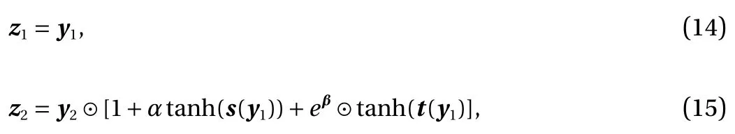
where α ∈(0,1) and β ∈Rn. First of all, the reformulated affine coupling layer adapts the trick of ResNet, where we separate out the identity mapping. Second, we introduce the constant α ∈(0,1) to improve the conditioning. It is seen from Eq. (7) that |det?yz|∈(0,+∞) for the original real NVP while (1?α)n?m≤|det?yz|≤(1+α)n?min our formulation. Our scaling can alleviate the illnesses when the scaling in the original real NVP occasionally become too large or too small. When α =1,|det?yz|∈(0,2). This case is actually similar to real NVP in the sense that the scaling can be arbitrarily small, and for wellscaled data by the scaling and bias layer, we do not expect a large scaling will be needed. When α =0, the formulation is the same as NICE, where no scaling is included. Third, we also make the shift bounded by letting it pass a hyperbolic tangent function.The reason for such a modification is similar to that for the scaling. The main difference here is the introduction of the trainable factor eβ. Compared to t (y1), eβdepends on the dataset instead of the value of y1, which helps to reduce the number of outliers for sample generation. Numerical experience show that our formulation in general works better than both real NVP and NICE. We usually let α =0.6.

Nonlinear invertible layer.It is seen that the affine coupling layer is linear with respect to the variable to be updated. We introduce component-wise nonlinear invertible mapping to allevimulative distribution function of a random variable defined on ate this limitation. We consider an invertible mapping y=F(x)with x ∈[0,1] and y ∈[0,1], where F (x) can be regarded as the cu-[0,1]. Then we have

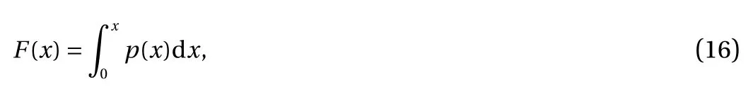
where p(x) is a probability density function. Let 0=x00. On [ ?a,a], we implement y=F[(x+a)/(2a)]followed by an affine mapping 2 ay ?a. In other words, we maps the domain to [0 ,1], and then map the range back to [? a,a]. On(?∞,?a) and ( a,∞), we just let y =x. Since the scaled data will be roughly centered at the origin, we only need to choose a sufficiently large a to cover the data instead of the whole real axis. In summary, we consider a mapping from R to R, where the mapping is nonlinear on [ ?a,a] and an identity mapping on(?∞,a)∪(a,∞).

We subsequently present some numerical experiments. For clarity we will turn off the rotation layers and the nonlinear invertible layers to focus on the effect of the triangular structure of KRnet, which provides the main improvement of performance.Let Y ∈Rnhave i.i.d. components, where Yi～Logistic(0,s). Let y[i:(i+k)]=[yi,yi+1,...,yi+k]T. We consider the data that satisfy the following criterion:

where

which is a product of a scaling matrix and a rotation matrix.Simply speaking, we generate an elliptic hole in the data for any two adjacent dimensions such that Yibecome correlated. Let Θi=π/4, if i is even; 3 π/4, otherwise. Let α =3, s =2, and C =7.6.For the training process we minimize the cross entropy between the model distribution and the data distribution

where μmodel(dy)=pY(y)dy , N is the size of training dataset and Θ are the parameters to be trained. This is equivalent to minimize the Kullback?Leibler (KL) divergence or to maximize the likelihood. To evaluate the model, we compute the KL divergence

where μtrueis known. First, we generate a validation dataset from μtruewhich is large enough such that the integration error in terms of μmodelis negligible. Second, we compute an approximation ofin terms of Y, where Y indicates the random variables that correspond to N samples in the training dataset. We take 10 independent training datasets.For each dataset, we train the model for a relatively large number of epochs using the Adam (the name Adam is derived from adaptive moment estimation) method [19]. For each epoch, we compute DKL(μtrue∥μmodel) using the validation dataset.We pick the minimum KL divergence and compute its average for the 10 runs as an approximation ofWe choose 10 runs simply based on the problem complexity and our available computational resources.

We first consider four-dimensional data and show the capability of the model by investigating the relation between N , i.e.,sample size, and the KL divergence. We let L =12, and K =3, in other words, one dimension will be deactivated every 12 general coupling layers. In, k =1,2,3, the neural network Eq. (5) has two hidden layers each of which has m rk?1neurons with m=24 and r =0.88. The Adam method with 4 mini-batches is used for all the training processes. 8000 epochs are considered for each run and a validation dataset with 1 .6×105samples is used to compute DKL(μtrue∥μmodel). The results are plotted in Fig. 2, where the size of training dataset is up to 8000. Assume that there exist a Θ0such that μmodel(Θ0) is very close to μtrue. We expect to observe the convergence behavior of maximum likelihood estimator, i.e.,～N?1/2, whereis the maximum likelihood estimator. It is seen that the KL divergence between μtrueand μmodel() is indeed dominated by an error of O (N?1/2). This implies that the model is good enough to capture the data distribution for all the sample sizes considered.

We subsequently investigate the relation between the KL divergence and the complexity of the model. The results are summarized in Fig. 3, where the degrees of freedom (DOFs) indicate the number of unknown parameters in the model. For comparison, we also include the results given by the real NVP. The configuration of the KRnet is the same as before except that we consider L = 2, 4, 6, 8, 10, and 12. The size of the training dataset is 6.4×105and the size of the validation dataset is 3 .2×105. We use a large sample size for training dataset such that the error is dominated by the capability of the model. For each run, 8000 epochs are considered except for the two cases indicated by filled squares where 12000 epochs are used because L is large. It is seen both the KRnet and the real NVP demonstrate an algebraic convergence. By curving fitting, we obtain that the KL divergence decays of O () for the KRnet and of O () for the real NVP, implying the KRnet is much more effective than the real NVP.

We finally test the dependence of the convergence behavior of the KRnet on the dimensionality by considering an eight-dimensional problem. We let K =7, i.e., the random dimensions are deactivated one by one. In, k =1,2,...,7, the neural network Eq. (5) has two hidden layers each of which has mrk?1neurons with m =32 and r =0.9. For each run, 12000 epochs are considered. All other configurations are the same as the four-dimensional case. The results are plotted in Fig. 4, where we obtain an overall algebraic convergence of O (N) in terms of DOF for L = 2, 4, 6, 8, and 10. It appears that the rate is not sensitive to the number of dimensions.

Fig. 2. KL divergence in terms of sample size for the four-dimensional case

Fig. 3. KL divergence in terms of DOFs of the model for the four-dimensional case

Fig. 4. KL divergence in terms of DOFs of the model for the eightdimensional case

In this work, we have developed a generalization of the real NVP as a technique for density estimation of high-dimensional data. The results are very promising and many questions remain open. For example, the algebraic convergence with respect to the DOFs is only observed numerically. The dependence of accuracy on the sample size is not clear although the convergence rate seems not sensitive to the dimensionality. These questions are being investigated and the results will be reported elsewhere.

Acknowledgement

X.L. Wan's work was supported by the National Natural Science Foundation of Unite States (Grants DMS-1620026 and DMS-1913163). Q.F. Liao's work is supported by the National Natural Science Foundation of China (Grant 11601329).