School of Mathematics and Statistics,Shandong Normal University,Jinan 250014,China

E-mail:guangzhidu@gmail.com

Abstract In this article,two kinds of expandable parallel finite element methods,based on two-grid discretizations,are given to solve the linear elliptic problems.Compared with the classical local and parallel finite element methods,there are two attractive features of the methods shown in this article:1)a partition of unity is used to generate a series of local and independent subproblems to guarantee the final approximation globally continuous;2)the computational domain of each local subproblem is contained in a ball with radius of O(H)(H is the coarse mesh parameter),which means methods in this article are more suitable for parallel computing in a large parallel computer system.Some a priori error estimation are obtained and optimal error bounds in both H1-normal and L2-normal are derived.Finally,numerical results are reported to test and verify the feasibility and validity of our methods.

Key words Two-grid method;expandable method;partition of unity;parallel algorithm;finite element method

1 Introduction

In recent years,the development of efficient parallel computing for PDEs with high resolution has been an hot research topic.On the basis of the understanding of the local and global properties of a finite element solution to PDEs with high resolution,a new local and parallel approach[20,21],was first proposed for a class of linear and nonlinear elliptic boundary value problems by Xu and Zhou.This local and parallel finite element algorithm was further applied for the Stokes and Navier-Stokes equations by He et al.[12–14,18]and for the mixed Stokes-Darcy problems by Du et al.[7–9].The algorithm has low communication complexity and allows existing sequential existing codes to run in a parallel environment with little investment in recoding.

However,one disadvantage of these local finite element algorithms is that the finite element solution is in general discontinuous.To overcome this defect,the author in[20]modified the above method to ensure that the final approximation is continuous.Furthermore,some local finite element methods based on a partition of unity are proposed in[6,15,22–25]to derive the globally continuous solution by assembling all the local solutions via the flexible and controllable partition of unity functions.The partition of unity method[3,17]introduces us to a flexible and controllable way to implement domain decomposition and construct a global solution.There are many interesting works about the partition of unity method.For example,Hou et al.[15]developed an expandable local and parallel two-grid finite element scheme by considering the case of the Poisson equation,while for the computational fluid dynamic problems,Zheng et al.[22–25]proposed some new partition of unity methods based on two-grid discretiaztions and Appelhans et al.[2]proposed a new,low-communication algorithm for solving PDEs on massively parallel computers based on range decomposition.Larson et al.[16]and Song et al.[19]utilized the partition of unity method as the localization technique in post-processing procedure,and Bank et al.[4]presented a new domain decomposition algorithm for the parallel finite element solution of elliptic partial differential equations.

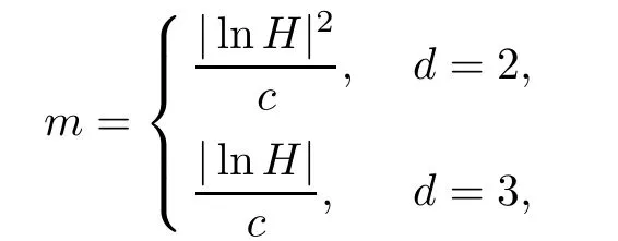
Although the partition of unity method could derive the globally continuous solution,the error estimates heavily depend on the usage of the superapproximation property of finite element spaces.As we known,the usage of this property causes the embarrassed problem that the distance between the boundaries of a specific subdomain and its expansion should be of constant order.Therefore the expansion of the subdomain could not be arbitrary small even when the diameter of the subdomain tends to zero.This will lead to a vast waste of parallel computing resources.In[15],we proposed an expandable local and parallel two-grid finite element scheme to overcome the dependence on superapproximation.The scale of each subproblem can be arbitrary small as H tends to zero and every two adjacent subproblems only have a small overlapping.Superposition principle is used to generate a series of local and independent subproblems and to make the global approximation continuous.In order to obtain an approximation with same accuracy as the fine mesh standard Galerkin approximation,a few iterations(O(|lnH|2)in 2-D or O(|lnH|)in 3-D respectively)are essential.

Following the idea in[15],two expandable two-grid parallel finite element methods are given to solve the linear elliptic problems.The first algorithm is one iterative form while the second method is one non-iterative form.As in[15],in order to derive optimal estimates,a few iterations(O(|lnH|2)in 2-D or O(|lnH|)in 3-D)are essential for the iterative method.However,for the non-iterative form,patches of diameter O(|lnH|2)H or O(|lnH|)H in 2-D or 3-D respectively are sufficient to guarantee the same accuracy as the fine mesh standard Galerkin approximation because errors decay exponentially with respect to the number of layers of elements in patches(see[11]for detail).Both the two algorithms can reach the same accuracy as the fine mesh standard Galerkin approximation in theoretical analysis and numerical simulation.

From the visual point of view,the non-iterative form has a similar approach except patch is a m-layer.But in practice,the non-iterative form needs only one global communication to derive the globally continuous approximation,while for the iterative form,in each iteration,one global communication is essential to reach the global approximation.That is the non-iterative form needs less communication than the iterative form.

The outline of this article is organized as follows.In Section 2,some preliminary materials and assumptions on mixed finite element spaces are provided.In Section 3,two expandable twogrid parallel finite element methods are presented.In Section 4,some a priori error estimation and optimal error bounds in both H1and L2-normal for the two algorithms are derived.In Section 5,some numerical experiments are reported to show the validity of our algorithms.Finally,a short conclusion is given.

2 Preliminaries

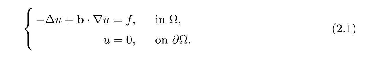
In this article,we consider the following linear elliptic equations with Dirichlet boundary condition defined in convex bounded domain ??Rd,d=2,3:

For a nonnegative integer s,we denote by Hs(?)the Sobolev space[1]in usual sense and their associated normswhile denote bythe closed subspace of H1(?)consisting of functions with zero trace on??.For convenience,the symbolsandwill be used in this article.Thatandmean thatandfor some constants C1,c2,c3,and C3independent of mesh size.For sub-domains S1? S2? ?,we write S1?? S2to mean that.

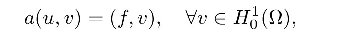
In the following,we denote by(·,·)the L2-inner product on ?.Thus,Let us define a(·,·)as a(u,v)=(?u,?v)+(b ·?u,v), ?u,where(·,·)is the standard inner-product of L2(?).Then,the weak formulation of(2.1)reads: findsuch that

A sufficient and necessary condition for the well-posedness of(2.2)is that

The variational problem(2.2)has a unique solution(see,for ample,[5]).Assume that a(u,v)is continuous,that is,

and coercive,that is,

For a given bounded domain ??Rd,we assume thatis a regular triangulation of ?.Here,is the mesh parameter.Associated with the mesh TH(?),letbe a C0- finite element space on ? andwhere r≥1 is a positive integer,andis the space of polynomials of degree not greater than r defined on

For these finite element spaces and problem(2.1),we make the following assumptions.

A1 Interpolation.There is a finite element interpolation IHdefined on SH(?)such that for any0≤m≤s≤r+1,

A2 Inverse Inequality.For any w ∈ SH(?),

A3 Regularity.For any f ∈ Hr?1(?),the solution of

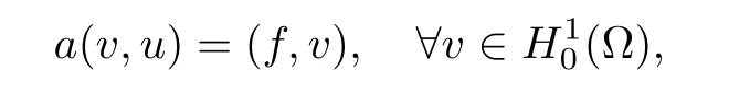
and its associated formal adjoint problem

satis fiy

Then,the standard Galerkin equation for solving(2.2)reads: findsuch that

For the standard Galerkin approximation uH,we have the following assumption:

which can be easily verified as long as u∈ Hr+1(?).

3 Numerical Algorithms

For each vertex xiof the coarse grid,let=supp φi=Di.We callthe patch of layer 0 defined on the ith vertex.Then,we can define the patch of layer m(m≥1,an integer)based on vertex i recursively.That is

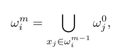
and the vertices on the boundary are included.For a proper chosen m,we denotesee Figure 1.For fine mesh parameter h,we introduce following fine mesh finite element spacesandwhich have the same definitions as SH(?)andgiven in the previous section.

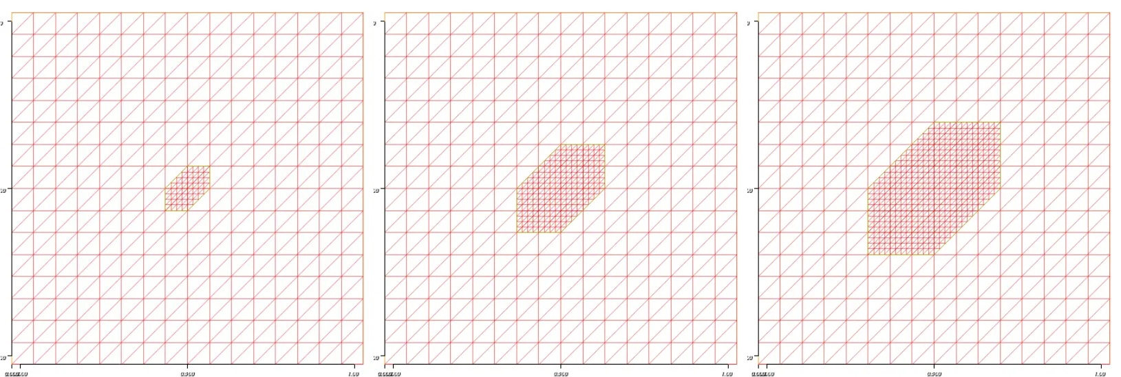
Figure 1 Patch of layer m(m=0,1,2),from left to right

Algorithm 1Iterative Form

1.Find a global coarse grid solutionsuch that

2.Find local fine grid correctionssuch that

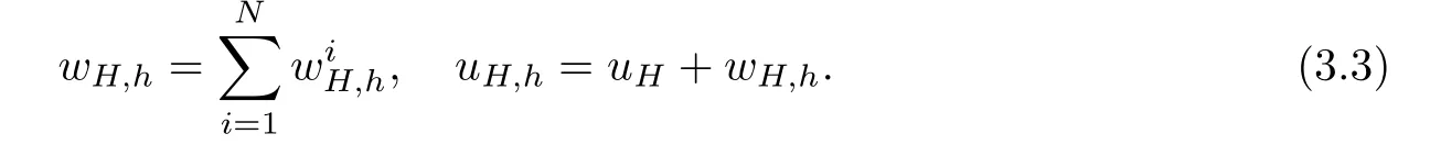
Set

3.Do a global correction on the coarse gird: findsuch that

And the final approximate solution is defined as

In the later numerical tests,it is easy to find that errors of the expandable two-grid parallel finite element method decay exponentially with respect to the number of layers of elements in patches.Therefore,for a proper chosen m,which is relevant to coarse mesh size H,it is sufficient to guarantee the same accuracy as the fine mesh standard Galerkin approximation.Let us denote,then we derive the following non-iterative form algorithm.

Algorithm 2Non-iterative Form

1*.Find a global coarse grid solutionsuch that

2*.Find local fine grid correctionssuch that

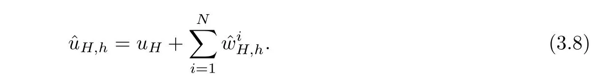
Set

3*.Do a global correction on the coarse gird: findsuch that

And the final approximate solution is defined as

RemarkIt is obvious that all the subproblems in Step 2 and 2*are independent,once the global coarse grid solution uHis known and the scale of each subproblem in Step 2 and 2*can be arbitrary small as H tends to zero and every two adjacent subproblems only have a small overlapping.The layer m in Step 2*is relevant to coarse mesh H(see Lemma 4.2*for detail).And the final finite element solutions in both forms are globally continuous.

4 Theoretical Results

In this section,we will give the theoretical results for Algorithm 1 and Algorithm 2.Firstly,we give the error estimates of Algorithm 1.

By the idea of fictitious domain method(see[10]),we extend the local sub-problem(3.2)to ?.Let us denote Γ = ?? and.Then,there existssuch that the zero extension ofsatisfies

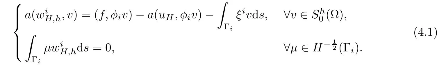
Denote

then the residual equation is

For the previously defined fine mesh Th(?)and the associated finite element spacethe Galerkin approximation for(4.2)reads:Findsuch that

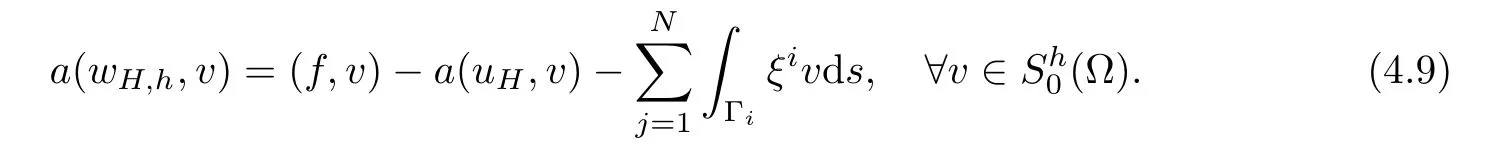
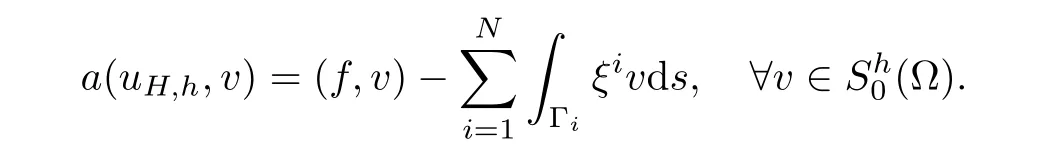
By the superposition principle,(4.3)can be rewritten as follows:Findi=1,2,···,N,such that

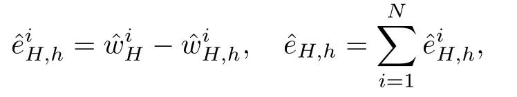
If we set the local error and the global error of uH,hby

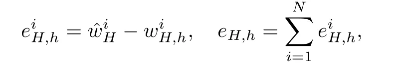
respectively,it is easy to obtain the following equations

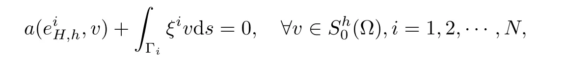
and

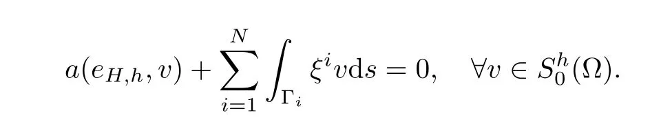
For all points x ∈ ?,it is clear that there exists a positive integer κ,which has nothing to do with N and x,such that each x belongs to κ differentat most.The following lemma can be found in[15].

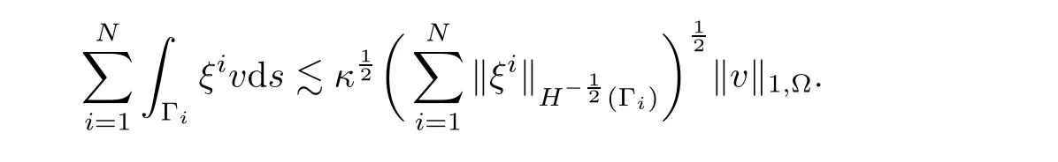
Lemma 4.1The multiplier ξiin(4.1)satisfies

and

Noting that

Thus,we obtain

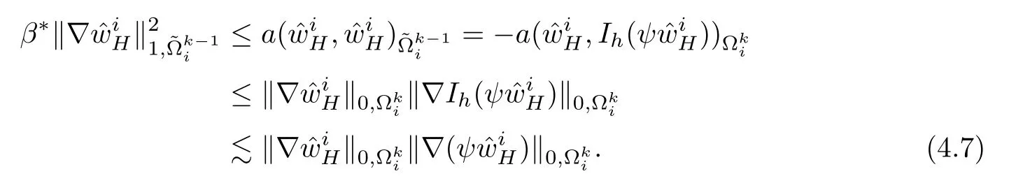
By(4.5),we give the estimate ofwhich plays a crucial role in the following section.

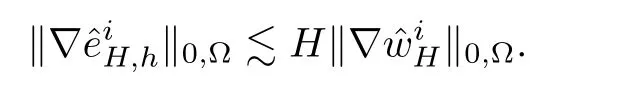
Lemma 4.2Let us set

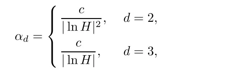
where c>0 is a positive constant that does not depend on H,h.Then,there holds

ProofLet us denote

and a series of disjoint annular zones

It is obvious that

Let us define

Noting that

Here,we introduce a smooth functionsuch thatfor k≥1 and

Because of the estimation ofin[15],there holds

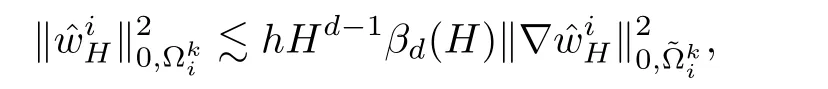
where βd(H)=H?1when d=3 and βd(H)=|lnH|when d=2.

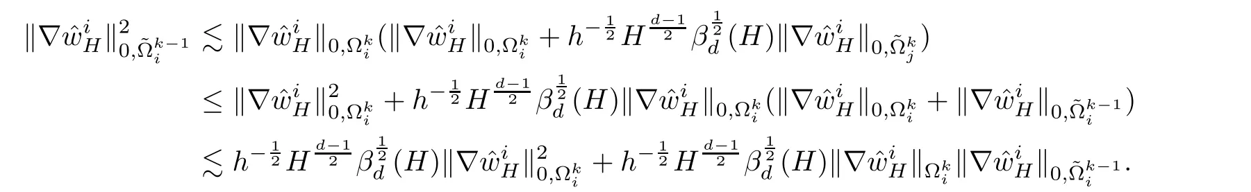
By Young’s inequality,we get

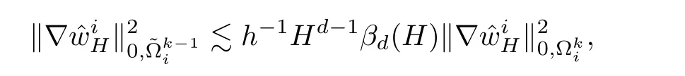
or

where c>0 is a constant that does not depend on H,h,i,and k.

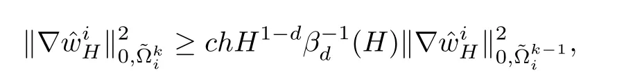
By repeating the last inequality,we have

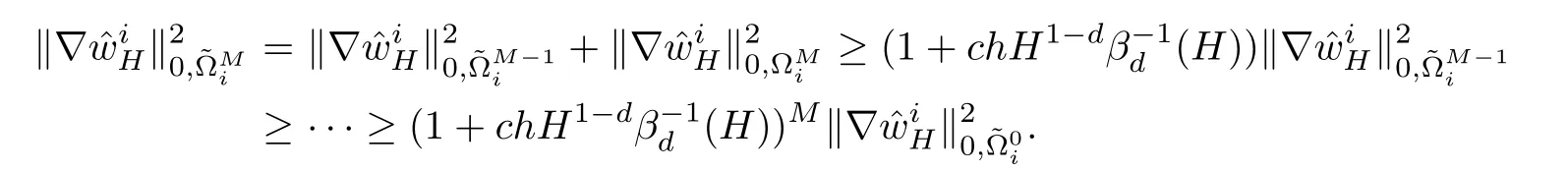
Therefore,

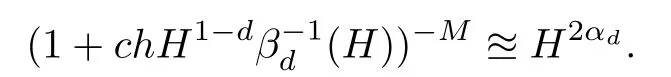
This,together with(4.5),concludes the proof of Lemma 4.2.

Following the result in Lemma 4.2,we have to give some estimates ofto estimate

Lemma 4.3Suppose that the assumptions A1–A3 are valid.Then,for i=1,2,···,N,we have

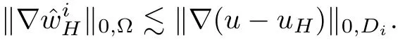
ProofUsing coercive property and takingin(2.5),we can obtain

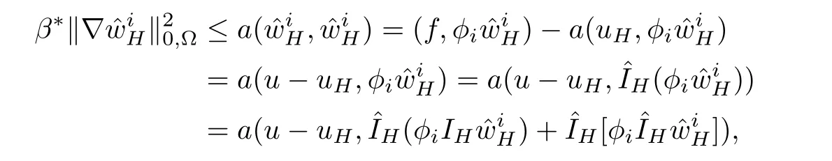
Using the continuity property of the bilinear form a(·,·),we have

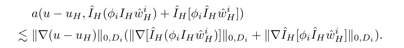
Assume that A1–A2 hold and notice that φiis a linear function on eachandthen we can obtain

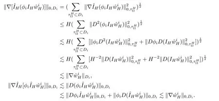
Adding the above two equations leads to

Now,we give the error estimations of Algorithm 1 in the following theorem.

Theorem 4.4Assume that assumptions A1,A2,A3,and(2.7)hold and u ∈ Hr+1(?).Then,

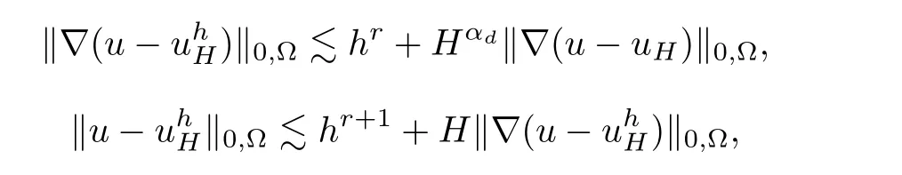
where αd>0 is defined in Lemma 4.2.

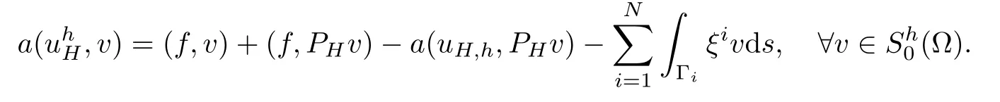
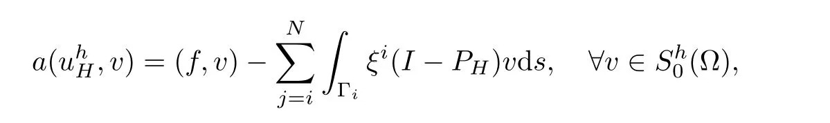
ProofAt the beginning,we introduce an H1-orthogonal projection PHfromonto:for givenfindsuch that

It is classical that

Hence,

On the other hand,the coarse mesh correction can be rewritten as

Combination of the above estimates yields

Finally,we have

and

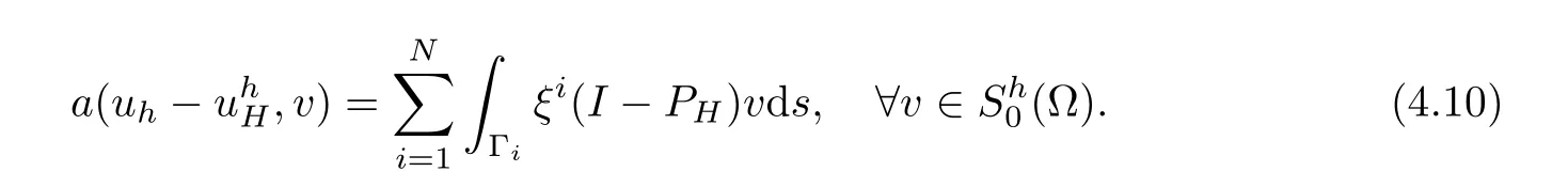
Using the above error equation ofand by Lemmas 4.1–4.3,we obtain

Because of the triangle inequality,we can easily derive the first result.

The Aubin-Nitsche duality argument is necessary for the L2-error estimate.Suppose that A3 is valid,then forthere existssuch that

and

Consequently,

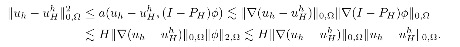
By combining triangle inequality,we finish the L2-error estimate.

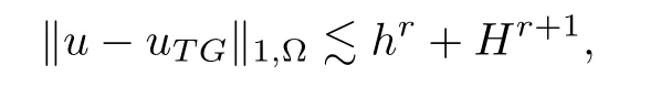
As our algorithms could be seen as varied two-grid methods,therefore,we expect our methods can reach the same convergence order with the two-grid method,which we called optimal error.

From the above results,it is easy to observe that we can improve the convergence order of both H1and L2errors of the coarse mesh standard Galerkin approximation uHfor αdorder by one two-grid iteration,and this phenomenon suggests us to do the following two-grid iteration with

? (Step 0)Let k=0 and solve(3.1)to obtainand we set;

?(Step 1)Solve the equations in(3.2)withto get,which are denoted byThen,we deriveby(3.3);

if k+1>K,stop the iteration and denotewhich is the final approximation with optimal error.Otherwise,let k:=k+1 and goto(Step 1).

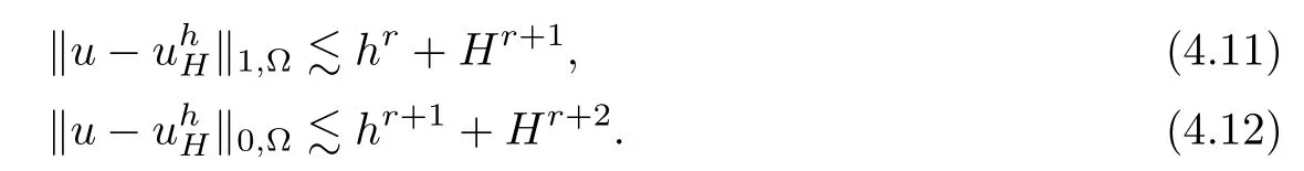
CorollaryAssume,the final approximationof scheme(Step 0)–(Step 2)has the following error estimates

Next,we give the the error estimations of Algorithm 2 in the same way.

Without distinction,we still use the same notions Γ = ?? and Γi= ?ωiΓ,and

the local error and the global error of uH,h,respectively.

It is obvious that Lemma 4.1 and Lemma 4.3 remain the same forms,while for Lemma 4.2,we do a little modification and get the following lemma.

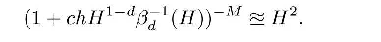
Lemma 4.2*For a proper chosen m,

where c>0 is a positive constant that does not depend on H,h,ωi.We have

ProofIn the same way,we have

This,together with(4.5),concludes the proof of the lemma.

Theorem 4.5Assume that assumptions A1,A2,A3,and(2.7)hold and u ∈ Hr+1(?).Then

5 Numerical Experiments

In this section,we will report some numerical examples(2D and 3D)to complement the analysis results.In the 2D experiments,the domain ? is the unit square ? =(0,1)× (0,1)with a uniform triangulationIn the 3D experiments,the domain ? is the unit cube ?=(0,1)3with a uniform triangulationP1element is employed for the finite element discretization.And all the following numerical results are obtained by using the public domain software FreeFem++.

5.1 2D-Example

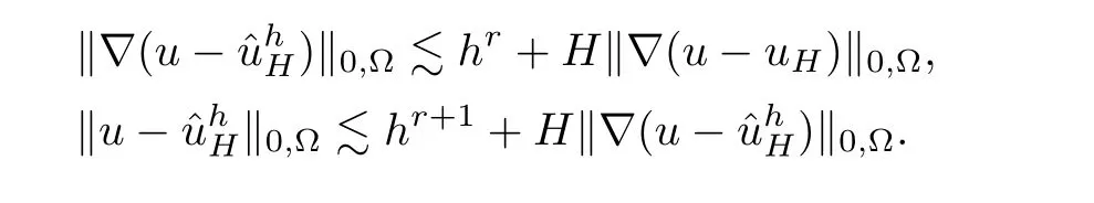
For both Algorithm 1 and Algorithm 2,to reach the H1accuracy,we should choose H and h such that h～H2.With such configuration,we have

On the other hand,to reach the L2accuracy,we should choose H and h such that h2～H3.In this case,

In the first experiment,we take b=(1.0,1.0)Tand consider the problem with the following analytic solution

Then,we can get f(x,y)in(2.1).

In the following Table 1 and Table 2,we give some numerical results according to the above configurations of H and h.For numerical experiments that the true solution u is known,we define the convergence order”O(jiān)RDER1” with respect to the coarse mesh size H as

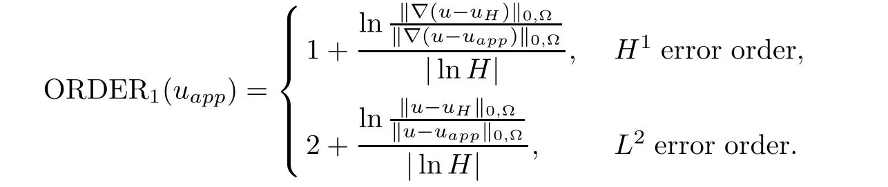
The symbol uappstands for certain approximation of u defined in the algorithms. “Iteration”stands for the number of iterations that are used for deriving the final approximation in Algorithm 1,and“m”stands for the patch of layer m that is necessary to obtain optimal error in Algorithm 2.

As seen from Table 1 and Table 2,both Algorithm 1 and Algorithm 2 reach almost the same accuracy as the fine mesh standard Galerkin approximation in H1-norm and L2-normal.For H1-normal,2 iterations are sufficient for Algorithm 1 and 2 patches of layer for Algorithm 2.Compared with the fine mesh standard Galerkin method,our algorithms can get better accuracy in L2-normal.

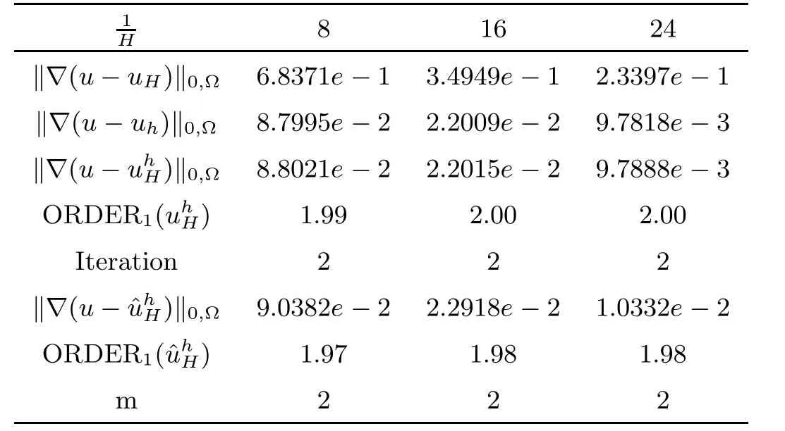
Table 1 H1-Error(h=H2)

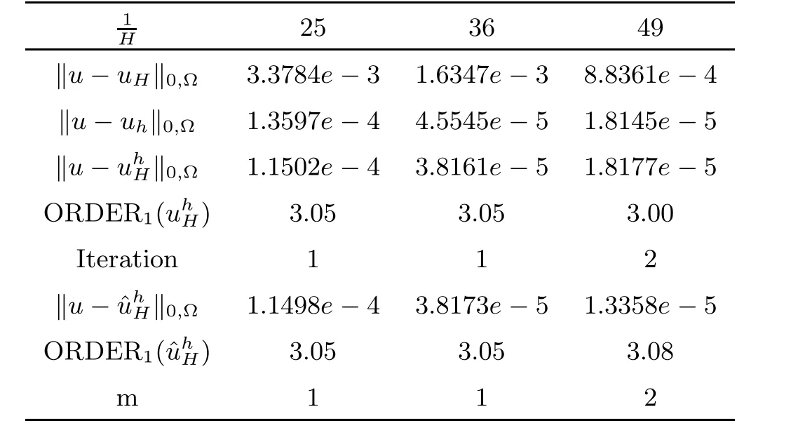
Table 2 L2-Error(h=H32)

In Figure 2,we show the evolution of error in H1-normal with “Iteration” (patch of layer)for Algorithm 1(Algorithm 2).It is clear that the error of Algorithm 1(Algorithm 2)decays rapidly with respect to “Iteration” (patch of layer).

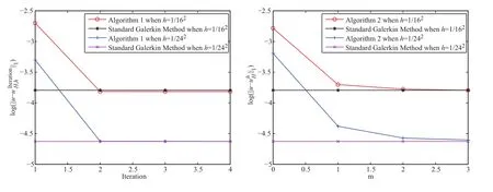
Figure 2 Left:evolution of error in H1-normal with “Iteration” for Algorithm 1;right:evolution of error in H1-normal with patch of layer for Algorithm 2

In the second example,we take b=(2x?ey,3y cos(πx))T,and f=70log((x+0.1)(sin(πy)+1))in(2.1).As the exact solution u is unknown,the convergence order of the approximate solution is calculated as

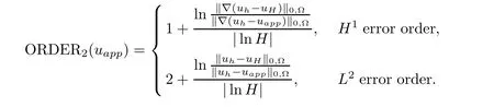
Here,uhis the standard Galerkin approximation in the fine mesh finite element spaceand the symbol uappstands for certain approximation of u defined in the proposed algorithms.It is generally known that the H1error estimate of the fine mesh standard Galerkin approximation admits the following estimation when h=H2

the “ORDER2(uapp)”calculated by the above formula equals to 2 means

therefore

Similarity,

The Table 3 and Table 4 report the numerical results of this test problem.It is clear that the errors obtained by the two algorithm are almost identical with each other and confirm the theoretical results.

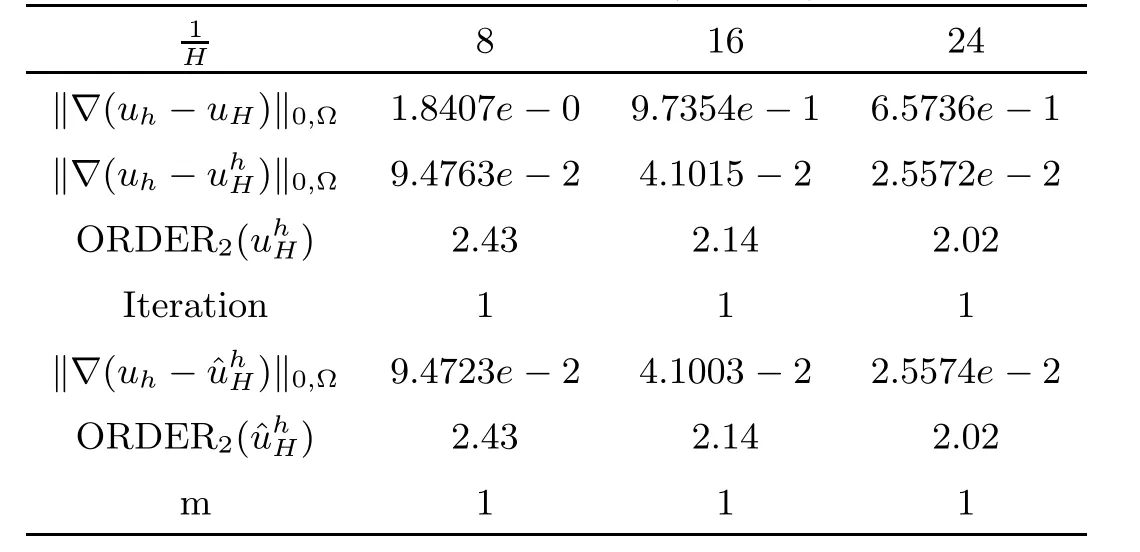
Table 3 H1-Error(h=H2)

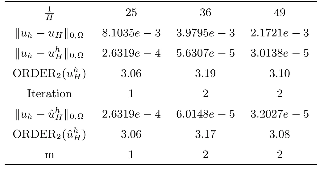
Table 4 L2-Error(h=H32)

5.2 3D-example

In this section,we will give two 3D examples.In these two examples,the domain ? is the unit cube(0,1)3and b=(1,1,1).In the first 3-D example,we consider the test problem with the the following analytic solution

The numerical results are given in Tables 5 and 6.

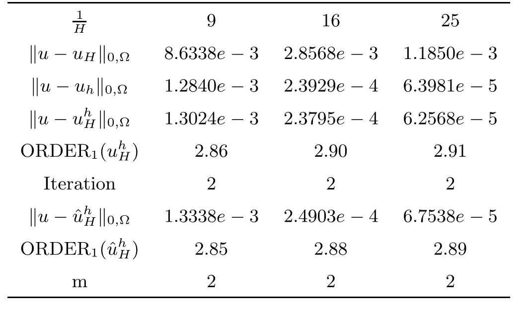
Table 6 L2-Error(h=H32)

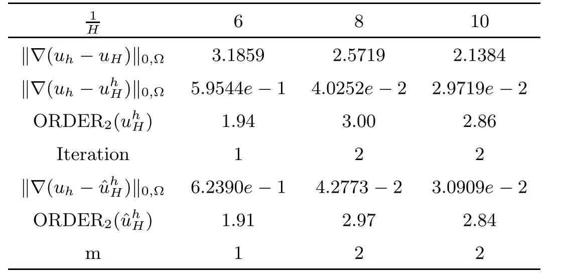
Table 7 H1-Error(h=H2)

Table 8 L2-Error(h=H32)

The second example of 3-D case is a test problem driven by the following free term

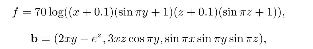
whose numerical results are given in Tables 7 and 8.

6 Conclusions

In this article,we have shown and analyzed two expandable two-grid parallel finite element methods for solving the linear elliptic problems.For Algorithm 1,a few iterations,sayor O(|lnH|)in 2-D or 3-D respectively,are essential to obtain optimal error;while for Algorithm 2,patches of diameter O(|lnH|2)H or O(|lnH|)H in 2-D or 3-D respectively are sufficient to guarantee to preserve the optimal convergence order.The numerical results and theoretical results keep consistent.Therefore,both the two algorithms can be regarded as flexible methods.