Mostafa M.A.Khater,Dian-Chen Lu, Raghda A.M.Attia, and Mustafa In?c

1Department of Mathematics, Faculty of Science, Jiangsu University, China

2Science Faculty, Firat University, 23119 Elazig, Turkey

Abstract This article studies the performance of analytical, semi-analytical and numerical scheme on the complex nonlinear Schr?dinger (NLS) equation.The generalized auxiliary equation method is surveyed to get the explicit wave solutions that are used to examine the semi-analytical and numerical solutions that are obtained by the Adomian decomposition method, and B-spline schemes (cubic, quantic, and septic).The complex NLS equation relates to many physical phenomena in different branches of science like a quantum state, fiber optics, and water waves.It describes the evolution of slowly varying packets of quasi-monochromatic waves, wave propagation, and the envelope of modulated wave groups, respectively.Moreover, it relates to Bose-Einstein condensates which is a state of matter of a dilute gas of bosons cooled to temperatures very close to absolute zero.Some of the obtained solutions are studied under specific conditions on the parameters to constitute and study the dynamical behavior of this model in two and three-dimensional.

Key words:complex NLS equation, generalized auxiliary equation method, adomian decomposition method,B-splines schemes (cubic & quintic & septic)

1 Introduction

Recently, the nonlinear partial differential equations have been used for modelling many complex natural phenomena such as giant permafrost explosions, desert roses,blood falls, bismuth crystals, synchronized hordes of cicadas, Salar de Uyuni, Pele’s hair lava, penitentes, aka fire tornadoes, fire whirls, halos, fire rainbows, volcanic lightning, and so on.Many analytical methods have been derived to study the explicit wave solutions of these complex phenomena that help in testing the accuracy of numerical schemes.It is also considered as a motivation for discovering more accurate numerical schemes that study the approximate solutions of these phenomena.For achieving this goal, the exact analytical wave solutions methods have experienced significant fast growth of development.Many methods have been derived to investigate the analytical and numerical solutions of many phenomena modeling such as modified exp (?Φ(ξ)) expansion method, generalized auxiliary equation method,(G′/G)-expansion method,Khater method,modified auxiliary equation method (modified Khater method), generalized Kudryashov method, generalized Riccati expansion method,generalized tanh-function method,improved Bernoulli subequation function, improved F-expansion method, sinh-cosh method, and so on.[1?15]

In 1925, Erwin Schr?dinger derived the famous nonlinear evolution equation and called it by a complex nonlinear Schr?dinger (NLS) equation.[16?25]The NLS equation relates with a quantum state, fiber optics, and water waves.The NLS illustrates the evolution of slowly varying packets of quasi-monochromatic waves,wave propagation,and the envelope of modulated wave groups, respectively for these branches.In the following lines,we mention some simple steps to show how this equation derived.

In studying of a particle in an infinite potential well,the particle of fixed energyEhas a wave function that can be represented as a linear next combination

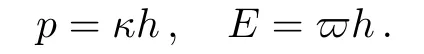
where Λ,(κ,?),x,t,and i are the amplitude of the wave,arbitrary constants,the positive direction,time,andrespectively.The momentum and energy of free particle can be expressed in the next formulas

So that, Eq.(1) can be rewritten as follows

Using the relation following betweenκ,h,p, andm:

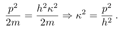
This relation leads to the next formula

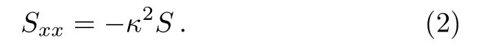
Similarly, we can write

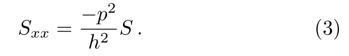
For both of a kinetic energy and a potential energy, we find

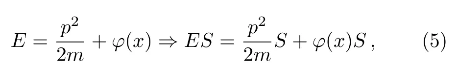
whereS, andφare wave, and potential functions, respectively.According to Eqs.(2), we have

Equation (6) is the nonlinear complex Schr?dinger equation.This equation takes many various formulas, we will mention some of them in the following equations

(i) Schr?dinger equation:

where

(ii) Nonlinear cubic Schr?dinger equation:

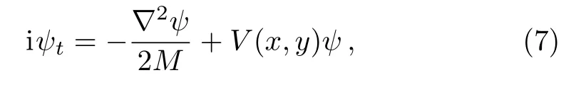
(iii) Nonlinear Schr?dinger equation:

(iv) Klein-Gordon-Schr?dinger equations:

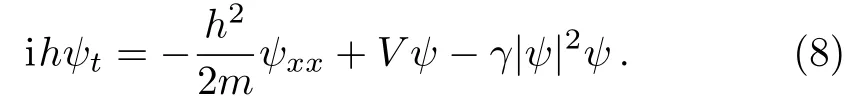
(v) Cubic-quintic Schr?dinger equation:

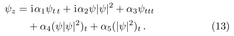
(vi) Perturbed nonlinear Schr?dinger equation:

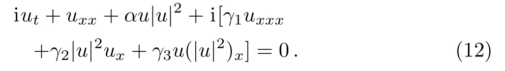
(vii) Higher-order nonlinear Schr?dinger equation:

Many various analytical solutions methods have been applying to these different forms of the famous NLS equation.In our paper, we select one of these forms and implement an analytical technique(generalized auxiliary equation method)[26?28]and four different numerical schemes (Adomian decomposition method, and B-spline schemes)[29?30]that never applied before to this form of the complex NLS equation to estimate the explicit wave solutions and the approximate solutions.This goal of this study is showing which one of these numerical schemes is more accurate than other.

Rest of the article is organized as follows.In Sec.2,we apply the generalized auxiliary equation method on the complex NLS equation.In Sec.3, we test our obtained solutions, by comparison, them with approximate solutions that obtained three numerical scheme.In Sec.5,we evince the conclusion of our paper.

2 Analytical Solutions

The complex NLS equation has the next formula

wherec=?2r.According to the generalized auxiliary equation method, the general solutions of Eq.(15) are in the next form

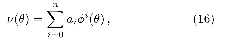
where?(θ) is the solution of the next ordinary equation

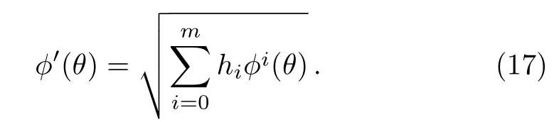
Balancing the terms in Eq.(15),we get a relation betweennandmin the following form

Takingn=2, leads tom=6.Thus, the general solution of Eq.(15) is in the next form

Substituting Eqs.(17) and (18) into Eq.(15) and collecting all coefficients of same power of?i(θ){i=0,1,2,...,6}, leads to a system of algebraic equations.Solving this system, we obtain

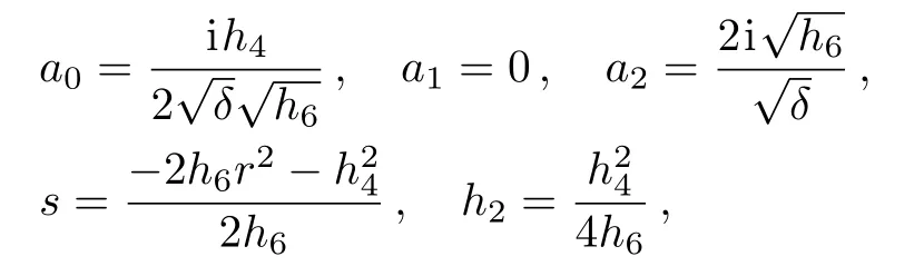
whereδ <0,h6>0.So that, the solitary wave solutions of Eq.(14) are in the next forms.

Family 1When,h0=h1=h3=h5=0:

Case 1When,h2>0

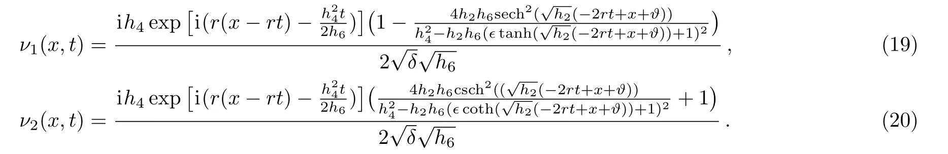
When,h2>0,h6>0

When,h2<0,h6>0

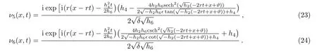
Family2When,h0=h1=h3=h5=0:

Case 1When,h24=4h2h6

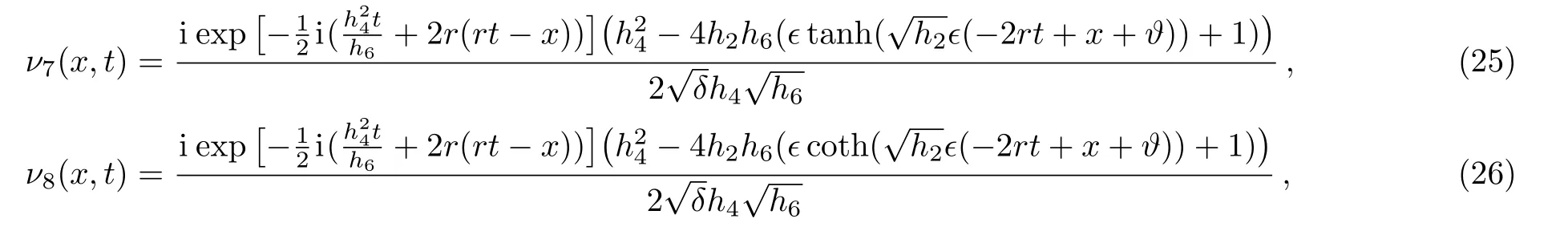
where?=±1.

3 Approximate Solutions

3.1 Adomian Decomposition Method

Applying the Adomian decomposition method to Eq.(25) allows obtaining the following solutions:

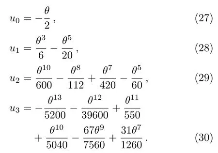
According to Eqs.(27)–(30), we get the approximate solution of Eq.(25) in the next formula

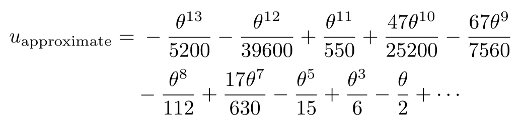
Now, we give a comparison between exact and approximate solutions at different points.

3.2 Cubic Splines

Using this kind of techniques allows putting the approximate solution of Eq.(25) in the next formula

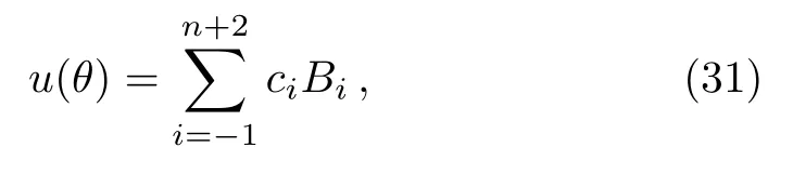
whereci,Bisatisfy the collection condition, respectively:Lu(θ)=f(θi,u(θi)),where (i=0,1,...,n).

where

we obtain

Substituting Eq.(33), its derivatives and boundary conditions of Eq.(25)into Eq.(15),gets(n+2)of equations.Solving this system of equations to get the value ofci, we obtain the following Table 2.

3.3 Quintic Splines

Using this kind of techniques allows putting the approximate solution of Eq.(25) in the next formula

whereci,Bisatisfy the collection condition, respectively:Lu(θ)=f(θi,u(θi)) where (i=0,1,...,n).

wherei ∈[?2,n+2], we obtain

Substituting Eq.(36),its derivatives and boundary conditions of Eq.(25)into Eq.(15),leads to(n+5)of equations.Solving this system of equations to get the value ofci, we obtain the following Table 3.

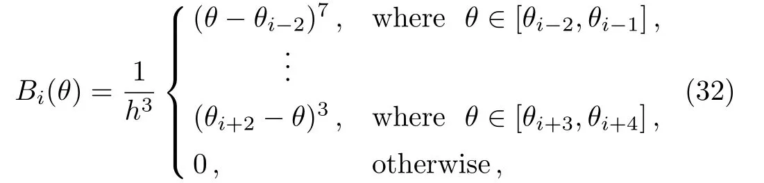
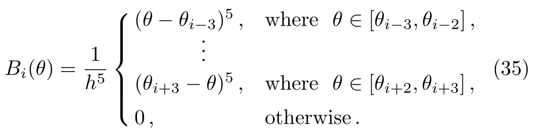
3.4 Septic Splines

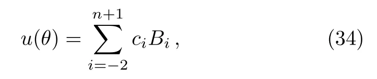
Using this kind of techniques allows putting the approximate solution of Eq.(25) in the next formula

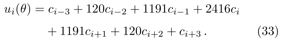
whereci,Bisatisfy the collection condition, respectively:Lu(θ)=f(θi,u(θi)) where (i=0,1,...,n).

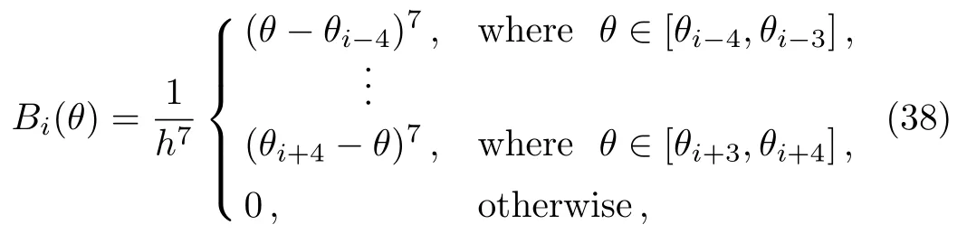
wherei ∈[?3,n+3], we obtain

Substituting Eq.(39), its derivatives and boundary conditions of Eq.(25)into Eq.(15),gets(n+7)of equations.Solving this system of equations to get the value ofci, we obtain the following Table 4.

4 Physical Explanation of Tables and Figures

In this section, we interest to clear of physical properties of our represented figures and tables.

4.1 Interpretation of Shown Tables

This part shows the mathematical and physical meaning of the shown tables as follows:

(i) Table 1 represents the convergence between the values of exact and approximate solutions.Moreover, it shows the fact of this method that is be more accurate when the value ofθnear to zero.

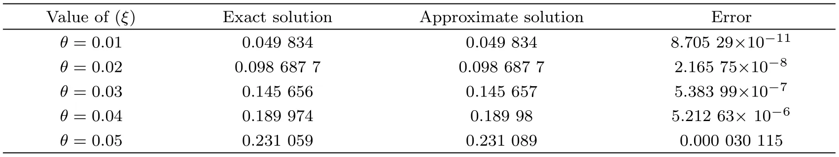
Table 1 Exact and approximate solutions of Eq.(15) at different value of θ to show the absolute error between both of them.

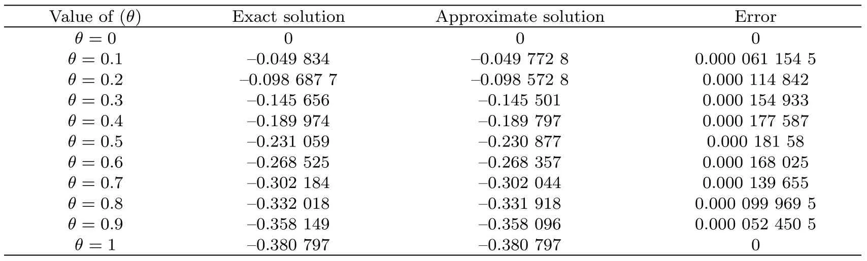
Table 2 Applying the cubic spline technique to determine exact and approximate solutions of Eq.(15) at different values of θ to study the absolute error of them.

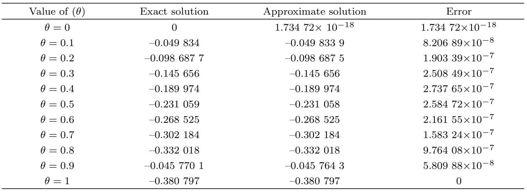
Table 3 Implementation of the quintic spline technique to determine exact and approximate solutions of Eq.(15) at various values of θ to represent the absolute error of them.

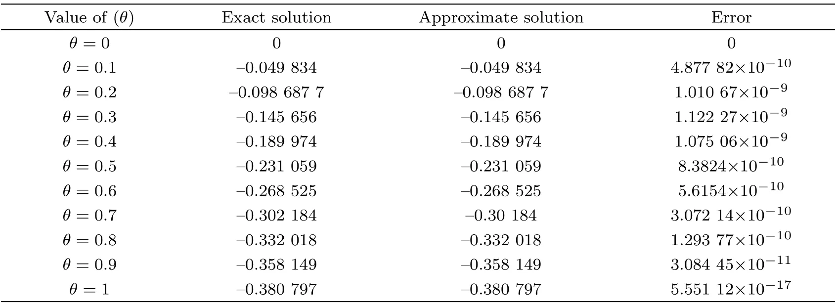
Table 4 Using septic spline technique to evaluate exact and approximate solutions of Eq.(15)at different values of θ to show the absolute error of them.

(ii) Table 2 gives the values of exact and approximate solutions at different values ofθthat show the values of the absolute value of error at the parties to the period are equal to zero and become bigger when taking away from the parties to the period until to reach to the middle of this period and come back again to decrease.

(iii) Table 3 aims to show the values of exact and approximate solutions for making a discussion about absolute error that is remarked that is increasing when the value ofθincrease.

(iv) Table 4 aims to show the values of exact and approximate solutions for making a discussion about the absolute error that is remarked that is increasing when the value ofθincrease.

4.2 Interpretation of Represented Figures

This subsection gives an interpretation of the shown figures in our paper.

(i) Figures 1–4 represent three and two-dimensional plots of Eqs.(25)and(26),when(δ=?4,h2=1,h6=4,h4=4,r=2,?=1,?=3).

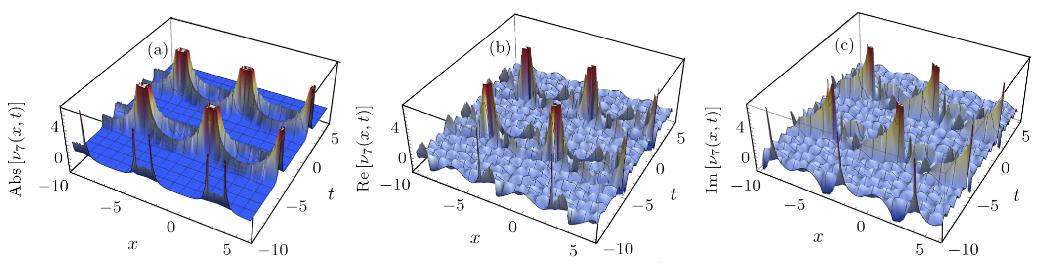
Fig.1 (Color online) Three-dimensional sketches for absolute, real, and imaginary solutions of Eq.(25), respectively.

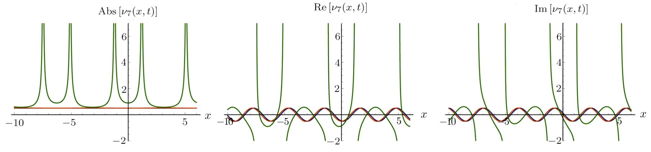
Fig.2 (Color online) Two-dimensional sketches for absolute, real, and imaginary solutions of Eq.(25), respectively.

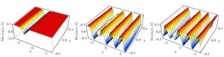
Fig.3 (Color online) Three-dimensional sketches for absolute, real, and imaginary solutions of Eq.(26), respectively.

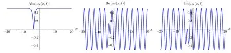
Fig.4 (Color online) Two-dimensional sketches for absolute, real, and imaginary solutions of Eq.(26), respectively.

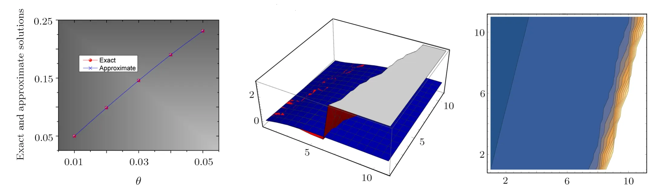
Fig.5 (Color online) List line plot in two and three-dimensional of Eqs.(25) and (31) and list contour plot of approximate solution (31).

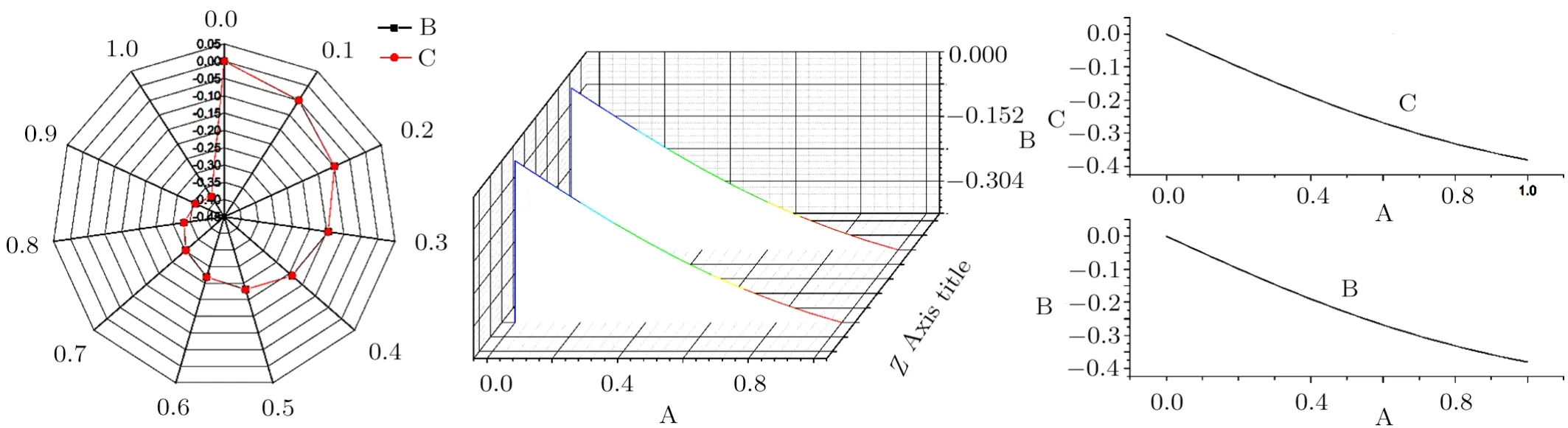
Fig.6 (Color online) Specialized radar, waterfall and verticals panel curves between exact and approximate solutions (25), (33).

(ii) Figure 5 shows the analytical and approximate solutions of Eqs.(25) and (31) via two and three-dimensional plots.We also represent the contour plot of approximate solutions (31).

(iii) Figure 6 represents the numerical that obtained by cubic spline and solitary solution of Eq.(14)via specialized radar, waterfall and verticals panel curves.

(iv) Figure 7 represents the line spline connected and specialized Radar plots for exact and numerical solutions that obtained by quintic spline.

(v) Figure 8 represents the list line plot, Pareto chart-Binned data, and scatter matrix curves for exact and numerical solutions that obtained by septic spline.

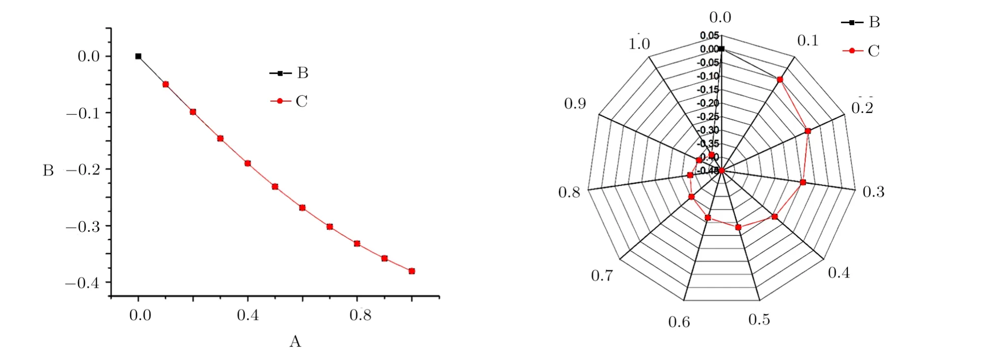
Fig.7 (Color online) Line spline connected and specialized Radar plots between exact Eq.(25) which represent by line (B), approximate Eq.(36) which represent by line (C) solutions and Error (B).

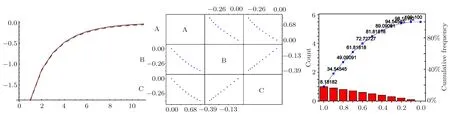
Fig.8 (Color online) List line plot, Pareto chart-Binned data and scatter matrix curves between exact and approximate solutions (25), (39).

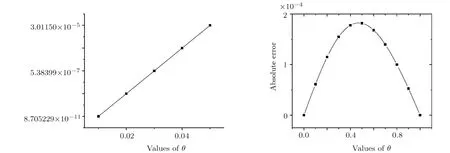
Fig.9 (Color online) Representation of absolute error for Tables 1–2.

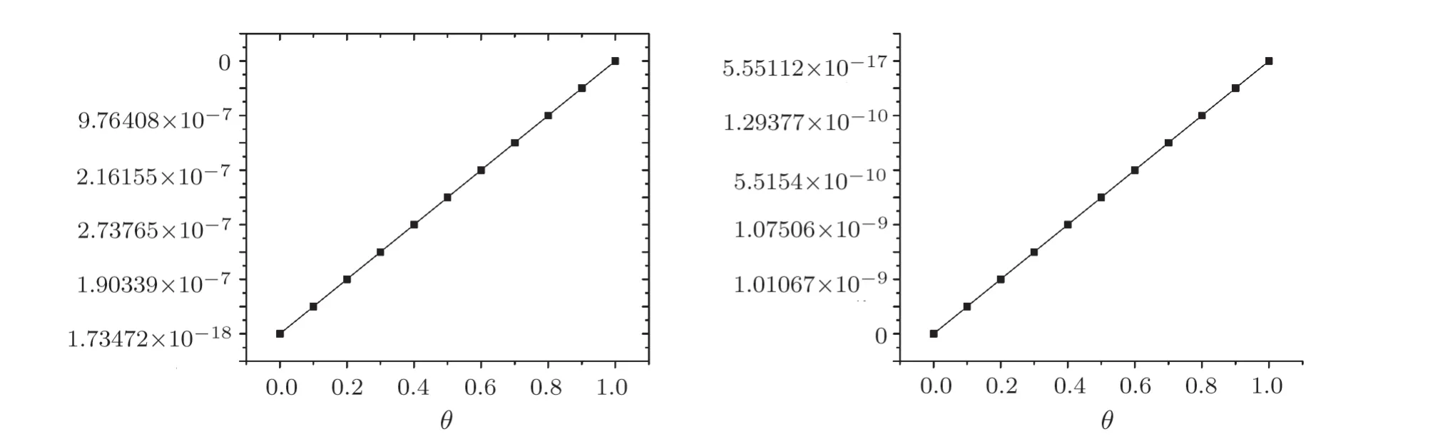
Fig.10 (Color online) Representation of absolute error for Tables 3–4.

5 Conclusion

This part of our paper gives a summary of the basic points in our paper.Analytical and numerical schemes have been successfully utilized to establish exact and approximate solutions of the complex NLS equation.Based on these five techniques, we got plenty of exact solutions that compared with four different approximate solutions to calculate the value of absolute error.Based on the values of the absolute errors that shown in Figs.9 and 10, we see that the Adomian decomposition method,quintic,and septic schemes obtained more accurate approximate solutions than cubic spline scheme.We also plot some figures to show how the difference between exact and approximate solutions are very tiny such that in some figures, we cannot recognize the difference between them.The obtained results will be helpful in different fields of science.