GUO Qidong(郭起東),CHEN Zhengzheng(陳正爭(zhēng))

(School of Mathematical Sciences,Anhui University,Hefei 230601,China)

Abstract: This paper is concerned with the large-time behavior of solutions to the Cauchy problem of the one-dimensional nonisothermal compressible Navier-Stokes-Korteweg system with density-dependent capillarity coefficient and temperature-dependent viscosity and heat conductivity coefficients,which models the motions of compressible viscous fluids with internal capillarity.If the corresponding Riemann problem of the compressible Euler system can be solved by a rarefaction wave,we prove that the 1D compressible Navier-Stokes-Korteweg system admits a unique global strong solution which tends to the rarefaction wave as time goes to infinity.Here both the initial perturbation and the strength of the rarefaction wave can be arbitrarily large.The proof is given by an elementaryL2 energy method.

Key words: Compressible Navier-Stokes-Korteweg system; Rarefaction wave; Global stability

1.Introduction

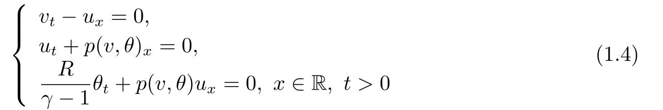
This paper is concerned with the Cauchy problem of the following one-dimensional compressible Navier-Stokes-Korteweg system in the Lagrangian coordinates:

with the initial and far field conditions:

Here the unknown functions are the specific volumev(t,x)>0,the velocityu(t,x),the absolute temperatureθ(t,x)>0,and the pressurep(v,θ) of the fluid,respectively,whileμ=μ(θ),κ=κ(v) and=(θ) denote the viscosity coefficient,the capillarity coefficient and the heat conductivity coefficient,respectively.v±>0,u±,θ±>0 are given constants and we assume that (v0,u0,θ0)(±∞)=(v±,u±,θ±) as compatibility conditions.

Throughout this paper,we assume that the pressurep(v,θ)and the constantCvare given by

wheresis the entropy of the fluid,andγ >1,AandRare positive constants.

System(1.1)can be used to model the motions of compressible viscous fluids with internal capillarity.The formulation of the theory of capillarity with diffuse interface was first studied by Van der Waals[1]and Korteweg[2],and then derived rigorously by Dunn and Serrin[3].Note that if the capillary coefficientκ=0,the system (1.1) is reduced to the compressible Navier-Stokes system.

There have been many results on the mathematical theory of the compressible Navier-Stokes-Korteweg system.For the case with small initial data,we refer to [6,9,12,14-15,17-18]and the references therein.For the case with large initial data,Bresch,Desjardins,and LIN[4]studied the global existence of weak solutions for an isothermal Korteweg system with a linearly density-dependent viscosity and a constant capillarity coefficient in a periodic domain Tdwithd=2 or 3.Haspot[11]proved the global existence of strong solution for an isothermal fluid with density-dependent viscosity and capillary coefficients in the whole space RNwithN ≥2.Charve and Haspot[5]showed the global existence of large strong solution to an isothermal Korteweg system with the viscosity coefficientμ(ρ)=ερa(bǔ)nd the capillarity coefficientκ(ρ)=ε2ρ?1in R (hereεis positive constant).Tsyganov[16]discussed the global existence of weak solutions for an isothermal system with the viscosity coefficientμ(ρ)≡1 and the capillarity coefficientκ(ρ)=ρ?5on the interval [0,1].Recently,Germain and LeFloch[10]investigated the global existence of weak solutions for the isothermal Korteweg system with general density-dependent viscosity and capillarity coefficients in R.Moreover,CHEN et al.[7?8]proved the global existence of smooth large solutions to the compressible Korteweg system in the whole space R with general density- and/or temperature-dependent viscosity,capillarity and heat conductivity coefficients.The time-asymptotic nonlinear stability of strong rarefaction waves for the isothermal Korteweg system with large initial data was also obtained in [7].

From the above results,it is easy to see that few results have been obtained on the global stability of basic waves for the compressible Navier-Stokes-Korteweg system so far.Here and hereafter,“global stability”means the nonlinear stability result with large initial perturbation.And if the initial perturbation is small,the nonlinear stability result is usually called“l(fā)ocal stability”.To our knowledge,there have been no result on the global stability of rarefaction wave to the nonisothermal compressible Navier-Stokes-Korteweg system up to now.This paper is devoted to this problem and we are concerned with the global stability of rarefaction wave for the Cauchy problem (1.1)-(1.2) with density-dependent capillarity coefficient and temperature-dependent viscosity and heat conductivity coefficients.

It is well-known that the large-time behavior of solutions to the Cauchy problem (1.1)-(1.2) is closely related to the Riemann solution of the compressible Euler system:

with the Riemann initial data

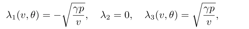
Then it is known that the Euler system (1.4) is a strict hyperbolic system of conservation laws with three distinct eigenvalues[25]:

and the Riemann problem(1.4)-(1.5)have two rarefaction waves solutions,denoted by(V r1,Ur1,Θr1)(t,x) and (V r3,Ur3,Θr3)(t,x),which are weak entropy solutions of (1.4)-(1.5) of the first and third family,respectively.

In this paper,we only consider the 1-rarefaction wave(V r1,Ur1,Θr1)(t,x),which is defined by

Since rarefaction waves are not smooth enough,to study the stability of the 1-rarefaction wave (V r1,Ur1,Θr1)(t,x),we need to construct its smooth counterpart.Letw(t,x) be the solution of the Cauchy problem of the Burgers equation:

withw±=λ1(v±,s?).Then we define the smooth approximate rarefaction waves(V,U,Θ)(t,x)of (V r1,Ur1,Θr1)(t,x) as follows:

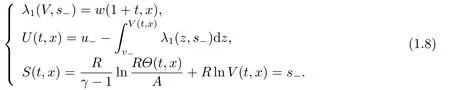
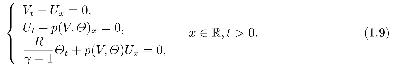
It is easy to check that (V,U,Θ)(t,x) satisfies:

The main result of this paper is as follows.

Theorem 1.1Let the condition (1.3) hold.Suppose further that the following conditions hold.

(i) The given constantsv±,u±,θ±do not depend onγ ?1;

(ii)The initial data(v0(x)?V(0,x),u0(x)?U(0,x),θ0(x)?Θ(0,x))∈H2(R)×H1(R)×H1(R) and

is bounded by some constant independent ofγ ?1;

(iii) There exist positive constantsandindependent ofγ ?1 such that

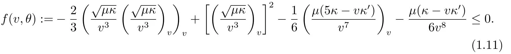
(iv)The viscosity coefficientμ(θ),the capillarity coefficientκ(v)and the heat-conductivity coefficient(θ) are smooth positive functions ofv >0 orθ >0,and the viscosity and capillarity coefficients are coupled by

Then there exist positive constantsδ0?1 andC0which depend only onand the initial dataN0such that the Cauchy problem (1.1)-(1.2) admits a unique global-in-time solution (v,u,θ)(t,x) satisfying

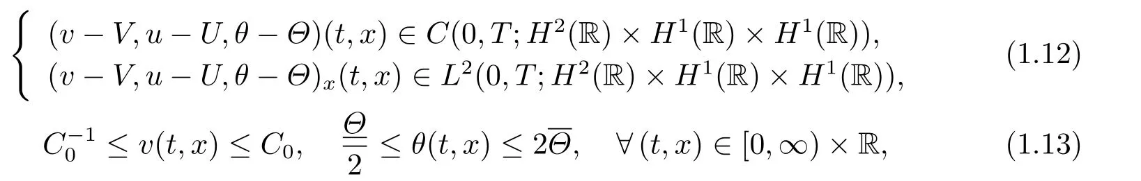
and the large-time behavior:

provided 0<δ:=γ ?1≤δ0.

NotesSome notes to Theorem 1.1 are given as follows.

1) The assumption (iv) is a technical condition in estimating(see the proof of Lemma 2.3 for details).

2) In Theorem 1.1,although the initial perturbation∥θ0(·)?Θ(0,·)∥H1(R)is small whenγ >1 is close to 1,the initial perturbations∥v0(·)?V(0,·)∥H2(R)and∥u0(·)?U(0,·)∥H1(R)can be arbitrarily large.Moreover,from the proof of Theorem 1.1,we see thatγ ?1 needs to be sufficiently small such thatwheref(N0) is a smooth increasing function on the initial dataN0(see(2.49)-(2.50)).Thus in this sense,Theorem 1.1 is a Nishida-Smoller type result[26]with large initial data.

3) It is interesting to study the global stability of some composite waves for the 1D nonisothermal compressible Navier-Stokes-Korteweg system,such as the combination of viscous contact wave with rarefaction waves,the combination of viscous contact wave with viscous shock waves,etc.,which is left for the future.

Before concluding this section,we remark that the nonlinear stability of basic waves for the compressible Navier-Stokes equations has been studied extensively.We refer to [19-20]] and the references therein for the nonlinear stability of viscous shock waves,[21-22] and the references therein for the nonlinear stability of rarefaction waves,and [23-24] and the references therein for the nonlinear stability of contact discontinuity.

The paper unfolds as follows.In the next section,we give the proof of our main Theorem 1.1,which is obtained by an elementaryL2energy method.

NotationsThroughout this paper,CandO(1)stand for some generic positive constants which may vary in different estimates.If the dependence need to be explicitly pointed out,the natationC(·,··· ,·) orCi(·,··· ,·)(i ∈N) is used.For function spaces,Lp(R)(1≤p ≤+∞)denotes the standard Lebesgue space with the normandHk(R) is the usualk-th order Sobolev space with its normFor simplicity,we denote the the norms∥·∥Hkand∥·∥L2by∥·∥kand∥·∥,respectively.

2.Proof of Theorem 1.1

This section is devoted to proving Theorem 1.1 and organized as follows.First,we reformulate our original problem (1.1)-(1.2) into a perturbation one around the approximate rarefaction wave and summarize the properties of the approximate rarefaction wave(V,U,Θ)(t,x)defined by(1.8).Then we focus on deducing the uniform-in-time energy estimates of solutions to the reformulate system(2.1)-(2.2).At the end of this section,we give the proof of the main Theorem 2.1 in this section,from which,we can get Theorem 1.1 immediately.

First,define the perturbation functions (?,ψ,ζ)(t,x) by

Then it is easy to get from (1.1) and (1.9) that

withx ∈R,t>0.System (2.1) is equipped with the following initial and far-filed conditions:

We define the solution space for the Cauchy problem (2.1)-(2.2) as follows:

wherem0,m1,M0,M1and 0≤T ≤+∞are some positive constants.

For the Cauchy problem (2.1)-(2.2),we have the following theorem,which together with Lemma 2.1 (iii) below implies Theorem 1.1 immediately.

Theorem 2.1Under the assumptions of Theorem 1.1,there exists a small positive constantδ0depending only onand the initial datasuch that the Cauchy problem (2.1)-(2.2) admits a unique global-in-time solution (?,ψ,ζ)(t,x)satisfying

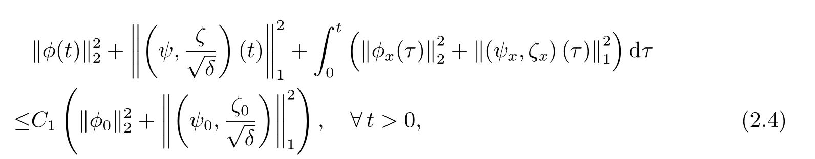
provided 0<δ:=γ ?1≤δ0.

Moreover,the following large-time behavior of solutions hold:

HereC0is a positive constant depending only onandis a positive constant depending only onand

In order to prove Theorem 2.1,we first give the local existence result.

Proposition 2.1(Local existence) Under the assumptions of Theorem 1.1,there exists a sufficiently small positive constantt1depending only onandsuch that the Cauchy problem (2.1)-(2.2) admits a unique strong solution (?,ψ,ζ)(t,x)∈and

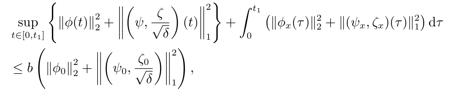
whereb>1 is a positive constant depending only onand

Proposition 2.1 can be obtained by using the dual argument and iteration technique,whose proof is similar to that of Theorem 2.1 in [12],and thus omitted here for brevity.

The global existence of solutions to the Cauchy problem (2.1)-(2.2) can be obtained by combining the local existence and the following a priori estimates.

Proposition 2.2(A priori estimates) Under the assumptions of Theorem 2.1,suppose that (?,ψ,ζ)(t,x)∈X(0,T;m0,M0,m1,M1) is a solution of the Cauchy problem (2.1)-(2.2)for some positive constantT >0,and satisfies the following a priori assumption:

for some positive constantN.Then there exist a positive constantC2depending only onm0,M0such that the estimates(2.3)-(2.4)hold for allt ∈[0,T],provided that the positive numberδ:=γ ?1 satisfies

To prove Proposition 2.2,we summarize some basic properties of the approximate rarefaction waves (V,U,Θ)(t,x) as follows lemma.

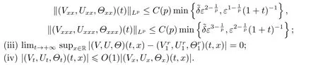
Lemma 2.1[22]Let=|v??v+|,then the approximate rarefaction waves(V,U,Θ)(t,x)satisfy the following:

(i)Vt=Ux>0,?x ∈R,t0;

The proof of Proposition 2.2 follows from a series of Lemmas below.First of all,notice that the a priori assumption (2.6) impliesfor allt ∈[0,T].Thus ifδ >0 is sufficiently small such thatthen we have

Consequently,

The following lemma concerns the basic energy estimates for the Cauchy problem (2.1)-(2.2).

Lemma 2.2There exists a positive constantsuch that

where the function Φ(·) is defined by Φ(s)=s ?1?lns.

ProofMultiplying the first equation in (2.1) bythe second equation in(2.1)byψ,and the third equation in(2.1)by,and adding the resultant equations together,we have

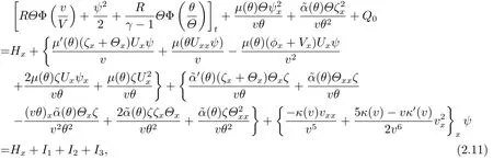
where

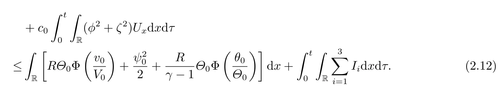
Integrating (2.11) over [0,t]×R yields

We derive from the Cauchy inequality,the a priori assumption (2.6) and Lemma 2.1 that

Similarly,

Using the first equation in (2.1) and integration by parts,we have

Similar to (2.13),we obtain

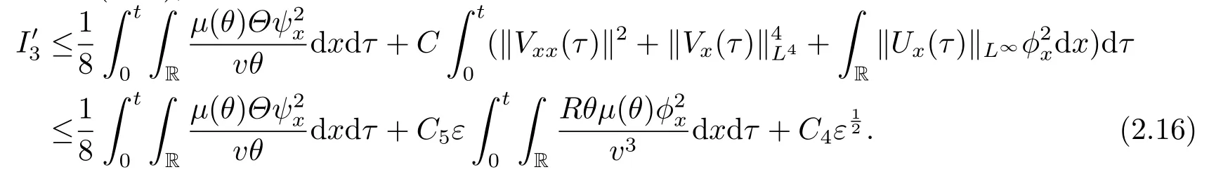
In the above estimates (2.14)-(2.16),C3,C4andC5are three positive constants depending only on

Combining (2.12)-(2.16),and using the smallness ofεsuch thatwe can get (2.10).This completes the proof of Lemma 2.2.

To control the reminder termdxdτin (2.10),we established the following lemma.

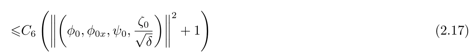
Lemma 2.3There exists a positive constantC2depending only onΘ,m0,M0and a positive constantC6depending only onsuch that

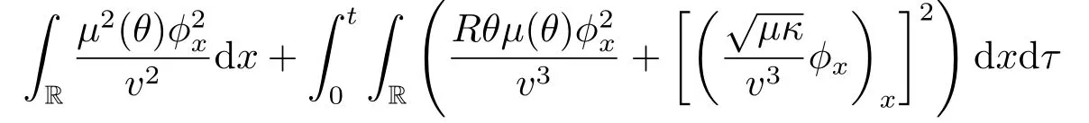
holds,provided

ProofNotice that

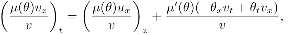
hence the second equation in (2.1) can be rewritten by

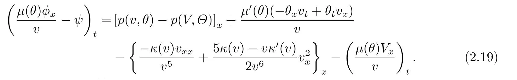
where

It follows from the third equation in (2.1),the Cauchy inequality and the Sobolev inequality that

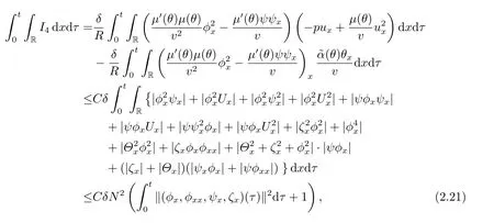
ForI8,we have

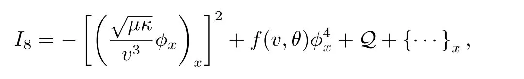
where

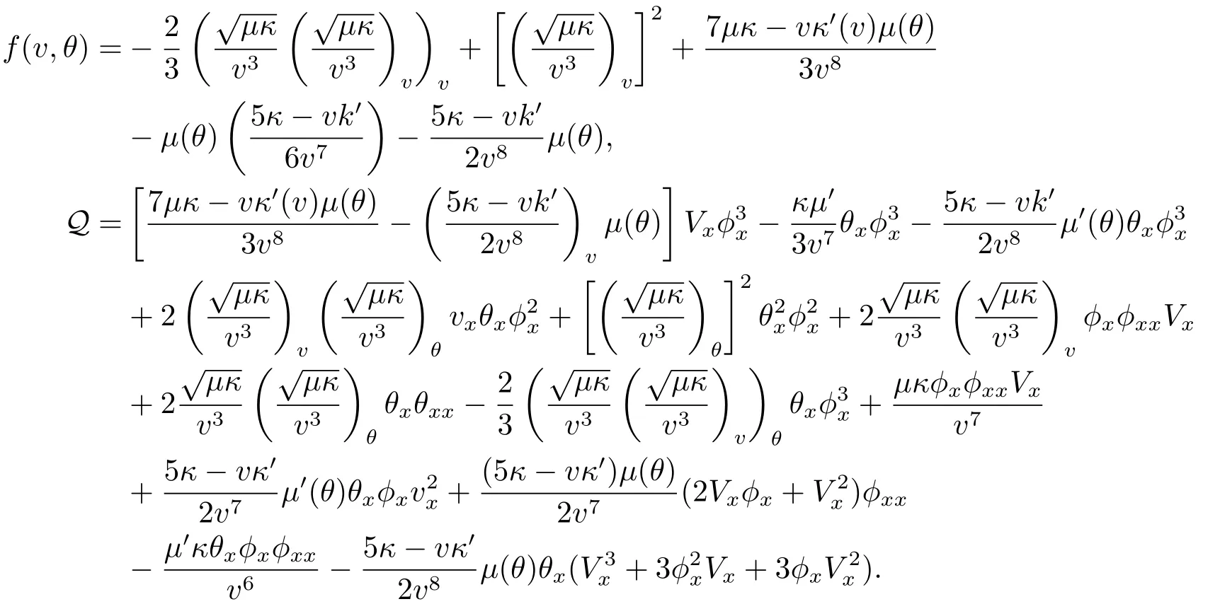
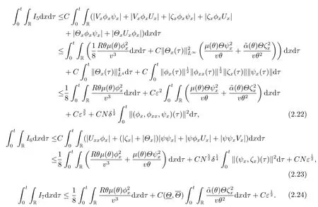
Similar to the estimates of (2.21)-(2.22),we have

Thus

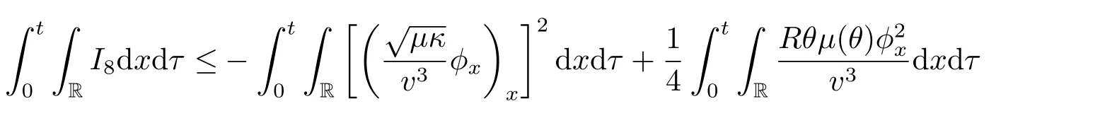
where we have used the assumption (1.11).

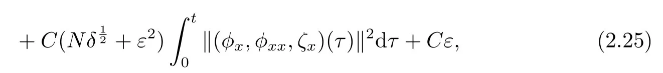
To estimate the reminder termin the above estimates,we rewrite

Consequently,it follows from (2.26),the Cauchy inequality and the Sobolev inequality that

which implies that

whereC7is a positive constant depending only on

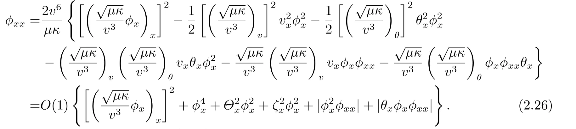
Combining (2.20)-(2.25) and (2.31),and using the Cauchy inequality,we obtain

whereC2is a positive constant depending only onm0,M0.

From (2.28) and Lemma 2.2,we have (2.17) holds provided thatδsatisfies (2.18) andεis sufficiently small such thatThe proof of Lemma 2.3 is finished.

Combining Lemmas 2.2-2.3 and (2.9),we have the following corollary.

Corollary 2.1Under the assumption of Proposition 2.2,there exists a positive constantsuch that

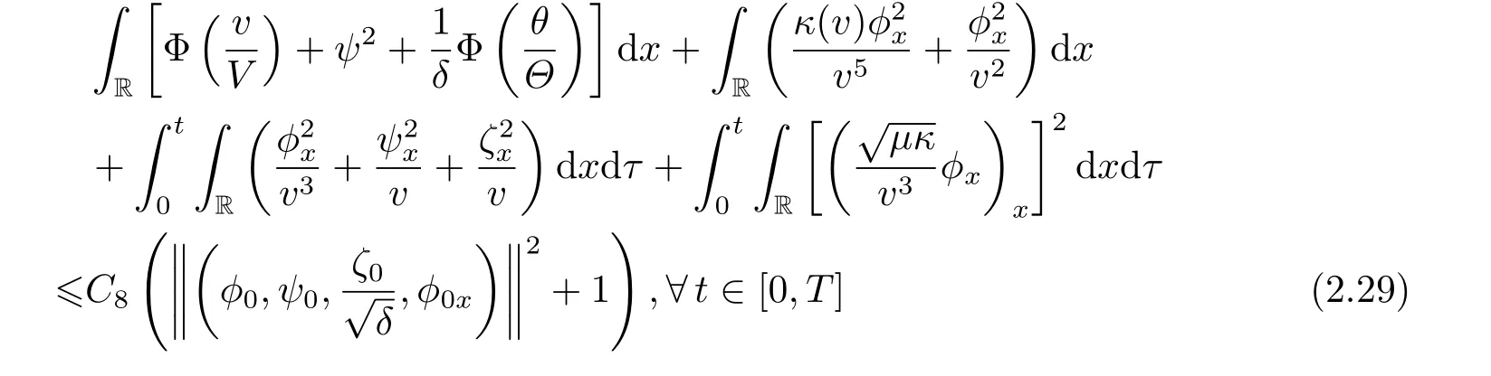
provided thatε>0 is sufficiently small.

Now we use Y.Kanel’s method[13]to deduce the lower and upper bound ofv(t,x).

Lemma 2.4Under the assumption of Proposition 2.2,there exists a positive constantsuch that

ProofLetand

Then there exist two positive constantsA1andA2such that

On the other hand,we have

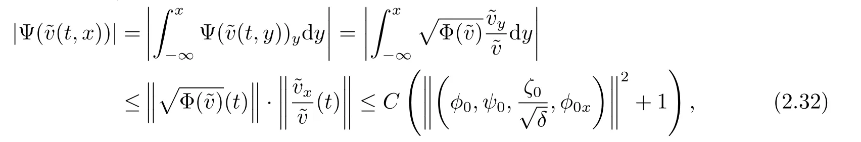
where we have used Corollary 2.1 and the following inequality

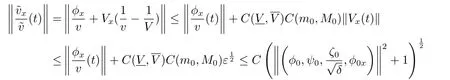
provided thatε>0 is sufficiently small.

Combining (2.31) and (2.32) yields

for allt ∈[0,T],whereC10,C11are two positive constants depending only onand

LettingC9=maxthen we have (2.30) holds.This completes the proof of Lemma 2.4.

As a direct consequence of Corollary 2.1 and Lemma 2.4,we have the following：

Corollary 2.2Under the assumption of Proposition 2.2,there exists a positive constantsuch that

ProofFirst,Corollary 2.1 and Lemma 2.4 imply that

whereC13is a positive constant depending only on

It follows from Corollary 2.1 and Lemma 2.4 that

Denoting the last term on the right hand side of (2.35) byI9,then by using the Cauchy inequality,the Young inequality and the Sobolev inequality,we have

Putting (2.36) into (2.35) gives

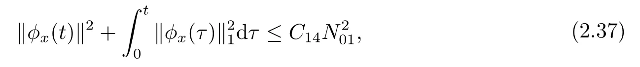
whereC14is a positive constant depending only onandN01.

(2.33) follows from (2.34) and (2.37) immediately.This completes the proof of Corollary 2.2.

Lemma 2.5Under the assumption of Proposition 2.2,there exists a positive constantsuch that

ProofMultiplying (2.1)2by?ψxx,and using (2.1)1,we have

Integrating the above equation over [0,t]×R,and using Lemma 2.4 and (2.9),we obtain

We derive from the Cauchy inequality,the Sobolev inequality,Lemma 2.4 and Corollary 2.2 that

Combining (2.39)-(2.42) yields

(2.43) together with the Gronwall’s inequality gives

whereC11,C12are two positive constants depending only onandN01.

Now,we turn to estimate∥ζx(t)∥.Multiplying the third equation in (2.1) by?ζxx,we have

Integrating(2.44)over[0,t]×R,and by repeating the same argument as above,we can obtain:

whereC16is a positive constant depending only onandN01.

Thus (2.38) follows from (2.44) and (2.46) immediately.This completes the proof of Lemma 2.5.

Lemma 2.6Under the assumption of Proposition 2.2,there exists a positive constant0 such that

ProofDifferentiating the second equation in (2.1) with respect toxonce,and multiplying the resultant equation bygives

where

Integrating (2.48) over [0,t]×R,similar to the proofs of Lemmas 2.4 and 2.5,we can get(2.47).The details are omitted here for brevity.This completes the proof of Lemma 2.6.

Proof of Proposition 2.2Proposition 2.2 follows from Corollary 2.2 and Lemmas 2.5-2.6 immediately.

Proof of Theorem 2.1Based on Propositions 2.1-2.2,we now use the continuation argument to extend the unique local solution (?,ψ,ζ)(t,x) to be a global one,i.e.,T=+∞.First,we have from Proposition 2.1 that (?,ψ,ζ)(t,x)∈X(0,t1;m0,M0,m1,M1) withm0=and the a priori assumption (2.6) holds with

for allt ∈[0,t1],wheret1>0 is a small positive constant given in Proposition 2.1.Then it is easy to find a small positive constantδ1>0 depending only onandN0such that

Thus if 0<δ=γ ?1≤δ1,then the inequalities in (2.3)-(2.4) hold for all (t,x)∈[0,t1]×R.

Now we take (?,ψ,ζ)(t1,x) as an initial data,then by Proposition 3.1 again,we can extend the local solution (?,ψ,ζ)(t,x) to the time stept=t1+t2for some suitably small constantt2>0 depending only onandN0.Moreover,(?,ψ,ζ)(t,x)∈X(t1,t1+t2;m0,M0,m1,M1)withand the a priori assumption(2.6)hold withThen there exists a small positive constantδ2>0 depending only onandN0such that

Consequently,if 0<δ ≤δ2,the inequalities in (2.3)-(2.4) hold for all (t,x)∈[t1,t1+t2]×R.Lettingδ0=min{δ1,δ2},then if 0< δ ≤δ0,the local solution (?,ψ,ζ)(t,x)∈X(0,t1+

Next,taking (?,ψ,ζ)(t1+t2,x) as initial data and using Proposition 3.1 again,we can extend the local solution (?,ψ,ζ)(t,x) to the time stept=t1+2t2.By repeating the above procedure,we can thus extend the local solution (?,ψ,ζ)(t,x) step by step to a global one provided that 0< δ < δ0.And as a by-product,the inequalities in (2.3)-(2.4) hold for all(t,x)∈[0,+∞)×R.

Moreover,the estimate (2.4) and the system (2.1) imply that

which together with (2.4) and the Sobolev inequality implies (2.5).This finishes the proof of Theorem 2.1.