Jia-zhong Qian (錢家忠), Ze-kun Wang (王澤坤), R. M. Garrard , Yong Zhang , , Lei Ma (馬雷)

1. School of Resources and Environmental Engineering, Hefei University of Technology, Hefei 230009, China

2. The 3rd Engineering Co., LTD of China Railway 16thBureau Group,Huzhou 313000, China

3. Department of Geological Sciences, University of Alabama, Tuscaloosa, Alabama, USA

4. State Key Laboratory of Hydrology-Water Resources and Hydraulic Engineering, Hohai University, Nanjing 210098, China

Abstract: A color visualization-based image processing method is developed in this paper to quantify the concentration evolution of the Brilliant Blue FCF transport through a two-dimensional homogeneous porous medium. A series of images are recorded at known time intervals, then the spatial distribution is estimated using a calibration curve, linking the gray pixel value to the solute concentration.Using a multi-dimensional concentration distribution map extraction technique the longitudinal and transverse concentration distributions could be observed with the physical model. The image-processed concentrations are then compared directly with the measured concentrations sampled at the outlet end. The tracer breakthrough curves sampled at multiple points along the central line of the medium are also compared with the solutions from the standard advection–dispersion equation model. It is shown that the non-invasive image processing method may be used to map the spatiotemporal evolution of a solute’s concentration without disturbing the flow or the transport dynamics, although the measured solute breakthrough curves feature some non-Fickian dynamics that cannot be efficiently captured by the standard transport model.

Key words: Solute transport, color tracer, porous media, image processing method

How to reliably quantify the contaminant transport in a porous media is one of the focuses of the hydrologic sciences as well as the closely related disciplines of geological sciences and petroleum engineering. The challenge is to accurately determine the solute concentrations and identify the pollutant dynamics in the system[1-2]. The ideal monitoring method should be non-invasive, so that the solute transport behavior can be continuously mapped in space and/or time. The mage analysis offers a great potential for the accurate and effective determination of the solute concentration in the porous media[3-7].This paper proposes a color visualization-based image processing method to give a quantitative determination of a tracer’s concentration in a two-dimensional porous media.

In order to improve the image quality and extract the effective information, a denoising treatment is essential. According to the literature[8], the median filtering is the best method to eliminate the random noise, which is used in this paper for denoising. The filter window is two-dimensional, with different shapes, such as linear, square, circular, and circular ring.

The two-dimensional median filter defined by Zhang[9]is briefly introduced here. The median value yijat point xijin the filter window A can be written as

where the operator “Med” means the median, andrepresents the gray value of each point of the digital image. Assuming that S is a neighborhood collection of the pixels surrounding the coordinate (x0,y0) (including (x0,y0)), (x, y) re-presents an element in the S, f( x, y) denotes the gray value at the point (x, y),represents the number of elements in the collection S, then a smooth processing can be expressed as

where the symbol “Sort” represents sequencing. The median filtering effect depends on two factors, the spatial extent of the neighborhood and the number of the pixels involved in the calculation of the mean value (when the space range is large, a sparse matrix is usually used in the calculation) with the advantage of being able to eliminate the random noise without bluring the edge.

The schematic setup is shown in Fig. 1. The experimental setup consists of three components,including a flow system, a Perspex box system, and an image-forming system. The flow system contains two Flexi glass flumes for the discharge/recharge and the flow rate adjustment. The dimension of the Perspex box is 480 mm×300 mm×10 mm (length×width×height), and the box is packed with uniform glass beads of 2 mm in diameter. The image-forming system contains multiple measurement devices, including a digital camera, a transformer, and a balance. We turn off other light sources in the laboratory, and set the light band under the model. The light emitted by the light band is uniformly distributed in the transparent organic glass plate of the model body, generating a uniform brightness for the captured image. To prevent any human impact on the stability of the photos, a tripod is fixed on the experimental bench, and the camera is then fixed on the tripod. We also adjust the tripod height and the camera parameters to ensure that the photo shoot is true and clear.

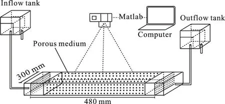
Fig. 1 Schematic diagram of the experimental setup

We then conduct the tracer experiment to obtain color images of the solute transport using the digital camera system built above. By analyzing the image information, the concentration distribution of the solute transport and the temporal evolution of the concentrations are obtained. They are shown in detail in the next section.

Changes in the image after denoising are shown in Fig. 2.

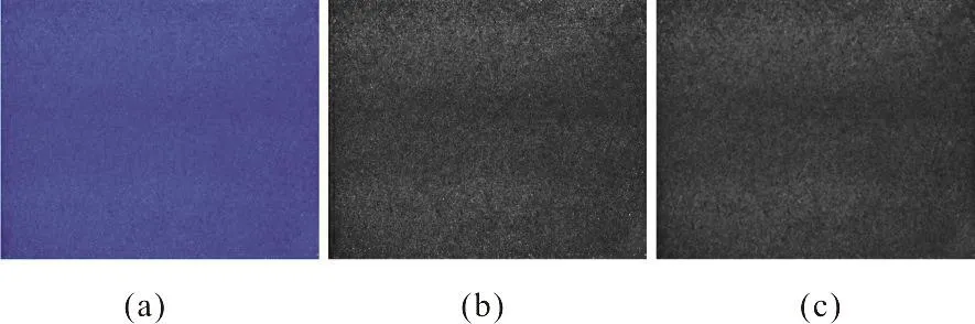
Fig. 2 (Color online) Denoising process

The median filter can remove the noise in the original image, but the change is actually very small.Therefore, we can obtain an accurate gray value for an image. A mathematical model is established to accurately and quickly build the relationship between the gray value and the concentration of the image. As shown in Fig. 3, the gray and concentration standard curve can be reliably established in a certain color space, where the gray level and the concentration are linearly correlated.

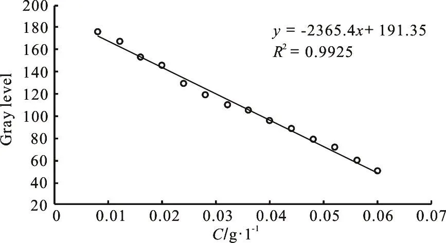
Fig. 3 Relationship between the gray level and the concentration measured in laboratory

Figure 4 shows a dimensionless concentration distribution and its corresponding 3-D map generated by MATLAB. Compared with the traditional sampling method, the imaging technology shows two apparent advantages. First, it does not cause a disturbance in the solute transport. Second, it demonstrates the concentration change over the whole surface not only at a few special points.

In order to check the feasibility of the imaging technology, we first compare the shot image with the measured concentrations. We sample the outlet BBF concentration by collecting samples at the outlet,without disturbing the internal water flow and the solute transport dynamics (Fig. 5). The directly measured BBF concentrations are found close to those obtained using the imaging process method (i.e., the concentrations converted from the gray value according to the transfer curve shown in Fig. 3).

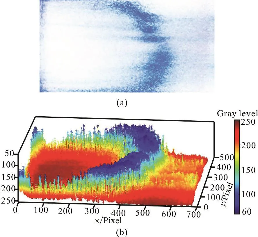
Fig. 4 (Color online) The 2-D/3-D concentration distribution map

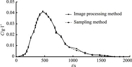
Fig. 5 Comparison between the shot image results with the measured concentrations

We then check the imaging technique with the model simulations. As shown in Fig. 6(a), we select three points along the central line and calculate their concentrations at each sampling time. The BTCs are compared with the model solutions. These BTCs represent the projected concentrations along the longitudinal direction, which may be approximated by the following one-dimensional ADE model

where C is the tracer concentration, and DLis the longitudinal dispersion coefficient. The initial condition is C( x, t=0)=M0δ(x)/θ where δ is the Dirac delta function. The left boundary is a reflective boundary where no tracers can exit via advection or dispersion, while the right boundary (at the outlet) is a free boundary.

The best-fit BTCs obtained by using (3) are shown in Fig. 6(b). The ADE model underestimates the late-time tail of the BTC. The discrepancy between the ADE solution and the measured BTC however is not surprising but well-documented in literature. The long tailing of the BTC[10-12]is a typical feature of the non-Fickian transport. Capturing the tailing of the BTCs is not the main focus of this study,and we will explore the non-Fickian dynamics in a future work. Figure 6(b) shows that, although the ADE model fails to capture the non-Fickian tailing, it does capture the overall trend of the solute transport,and indirectly supports the image processing technique developed in this study.

Fig. 6(a) The three sampling points at the center line

Fig. 6(b) Experimental data (symbols) versus the ADE model best-fit solution (lines) at the three sampling points

An image processing method is developed to identity the tracer concentrations in the two-dimensional porous media. The results obtained agree reasonably well with the traditional sampling approach of measuring the concentration directly at the medium’s outlet. Further analysis shows that the tracer breakthrough curves, at the central line of the medium,generally agree with the standard ADE model solutions, although the ADE model underestimates the BTC’s late-time tail due to its limitation in capturing the non-Fickian diffusion. The image processing method presented in this study therefore may provide a useful technique to monitor the spatiotemporal evolution of the contaminants moving through a twodimensional media without disturbing the dynamics of the water flow and the solute transport.