Guo Chai and Tian-jun Wang

Henan University of Science and Technology,Luoyang 471003,P.R.China.

Abstract.In this paper,we develop a spectral method for the nonlinear Fokker-Planck equations modeling the relaxation of fermion and boson gases.A full-discrete generalized Hermite spectral scheme is constructed.Its convergence and stability are proved strictly.Numerical results show the efficiency of this approach and coincide well with theoretical analysis.

AMS subject classifications:65M99,41A30,35K55

Key words:Nonlinear Fokker-Planck equations,the whole line,generalized Hermite spectral method,full-discrete scheme.

1 Introduction

In recent years,the more and more attentions were paid to the problems defined on unbounded domains.It is natural to take Hermite(or Laguerre)polynomial/functions as basis functions for the problems defined on the whole line(or half line),see for example[4,8,11,14,16,22,23,25,28,32,33].In earlier studies,with respect to the problems defined on the whole line,ones take the Hermite orthogonal polynomials with the weight function eλv2(λ is a non-zero constant)as the basis functions which lead to non-uniform weights.The non-uniform weights are not natural for certain underlying physical problems,see for example[1–3,10,11,13,17,19,26]and the references therein.In addition,for the problems with variable coefficients or nonlinear wave equations,such as the Fokker-Planck equations in statistic physics or Dirac equation in quantum mechanics,the solutions decay to zero at infinity.The non-uniform weights will destroy the symmetry and positive de finiteness of the bilinear operators as well as the conservation properties,and then lead to complications in analysis and implementation.In such cases,we prefer to consider approximations by Hermite functions with weight χ(v)≡1(see[15,24,31,34]).

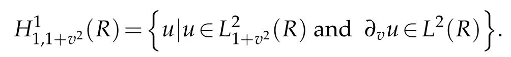
In this paper,we consider the Fokker-Planck equations modeling the relaxation of fermion and boson gases.Let v be the velocity of particles,R={v|?∞＜v＜∞}.Denote by W(v,t)the probability density.What’s more,W0(v)represents the initial state.For simplicity,letetc..We think of the following Cauchy problem(see[28]),

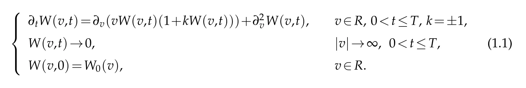
The Fokker-Planck equations have been put forward as kinetic models for the relaxation to equilibrium for bosons(k=1)and fermions(k=-1),see[5,9,20]and the references therein.These models have been introduced as a simplification with respect to Boltzmann-based models as in[7,21].Carrillo,Rosado,and Salvarani[6]indicated that inwhichway theentropymethodappliesforquantifying explicitly theexponentialdecay towards Fermi-Dirac and Bose-Einstein distributions in the one-dimensional case.Also,someauthors consideredFokker-Planck equationsin an in finite channel orthe whole line by using Laguerre functions coupled with domain decomposition(see[18,27,28]).The domain decomposition method needs much more basis functions and is extremely complicated to analyze and implement for the problems defined on unbounded domains.In particular,it costs a lot of work to match the numerical solutions on the common boundary of the adjacent subdomains.Thus it is more appropriate to consider approximations by Hermite functions Hσn(v)(see[31])directly.

This paperaims at expoundingonthegeneralized Hermitespectralmethodto thenumerical solution of problem(1.1).Firstly,the main difficulty in dealing with(1.1)numerically is caused by the two order difference terms of nonlinear?v(vW(v,t)(1+kW(v,t))).To estimate the errors rooted in the nonlinear terms,we need serval inverse inequalities.Next,we need a fewlemmas in time t-direction for numerical analysis of the full-discrete scheme of(1.1).In addition,the fact that the terms?2vW(v,t)and ?vW(v,t)in(1.1)possess thecoefficients 1 and v varying from?∞to∞,brings some difficulties inactual computation and numerical analysis(see[28]).To remedy the deficiency,we need a nonstandard projection of generalized Hermite functions(see[29]).Then a generalized Hermite spectral scheme for(1.1)can be constructed,and its convergence and stability can be proved too.Since in many cases,W(v,t)decays very fast as v→∞,it is better to use the generalized Hermite functions as the basis functions in actual computation(see[24,31]).They are L2(R)-orthogonal system with regard to weight χ(v)≡1,lead to a much simplified analysis,more precise error estimates and easier algorithms.We also design an efficient algorithm for actual computation,and present some numerical results showing the efficiency of this approach.

This paper is organized as follows.In Section 2,we introduce some results on the generalized Hermite approximation,which play important roles in the numerical analysis of spectral methods for various differential equations in an in finite interval.Then we construct the Hermite spectral scheme for(1.1)and prove its convergence and stability in Section 3.We present some numerical results indicating the high accuracy of the proposed algorithm in Section 4.The final section reveals some concluding remarks.

2 Preliminaries

In this section,we present some notations and basic results concerning the generalized Hermite orthogonal approximation which will be used in the sequel.

2.1 Generalized Hermite approximation

Let R={v|?∞＜v＜∞}and χ(x)be a certain weight function.For any integer r≥0,we define the space Hrχ(R)as usual,equipped with the inner product(u,v)r,χ,R,the seminorm|u|r,χ,R,and the norm‖u‖r,χ,Λ.In particular,(R)=(R),with the inner product(u,v)χ,R,and thenorm‖u‖χ,R.Thesubscript χ is omitedin thenotationswheneverχ(v)≡1.

Let Hn(v)be the usual Hermite polynomials,namely,

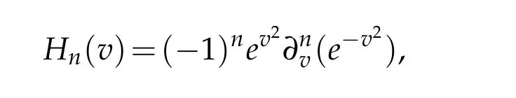
which are mutually orthogonal with the weight function χ(v)=e?v2.The generalized Hermite function of degree n is defined by(cf.[31])

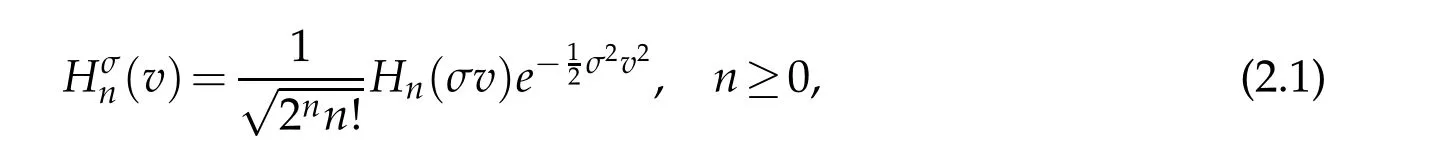
where σ＞0 is a constant.

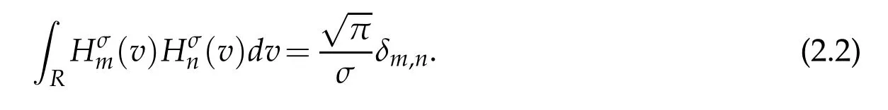
The set of generalized Hermite functions(v)forms a complete L2(R)-orthogonal system,namely,

with the corresponding eigenvalue λn= λn(n,σ):=2σ2n.According to Equation(2.4),Equation(2.5)of[31],we have

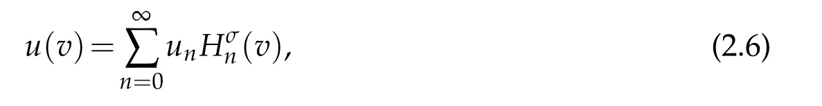
For any u∈L2(R),we can write

Thanks to Lemma 2.1 of[31],for any φ ∈ QN,σ(R)(cf.[15]for σ =1),

Lemma 2.1.For any φ ∈ QN,σ(R),we have that

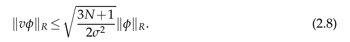
Proof.For any φ ∈ QN,σ(R),letBy(2.4),we get

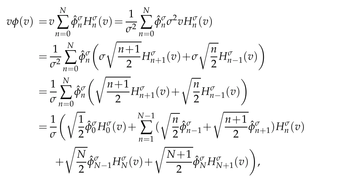
then,we have

The above derivation leads to the desired result.

We need the following inverse inequality which will be used in the forthcoming analysis.

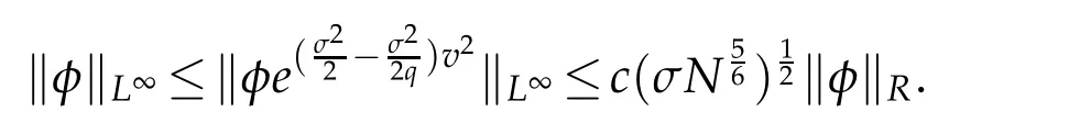
Remark 2.1.For any φ ∈QN,σ(R)and q≥1(cf.[34]),

In particular,

In order to represent the approximation results,we introduce a normed space(see[31]).For any integer r≥0,let

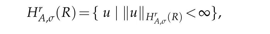
equipped norm

The orthogonal projection PN,σ,R:L2(R)→QN,σ(R),defined by

Proposition 2.1.If u∈(R)and integers 0≤μ≤r,then(cf.[31])

The above result with σ=1 was firstly given by Guo et al.,see Theorem 2.3 of[15].

We need a nonstandard projection which plays an important role in the forthcoming analysis.To do this,let

Proposition 2.2.If u∈and integer r≥1,then(cf.[29])

Lemma 2.2.For any u∈H1(R)(cf.[34]),

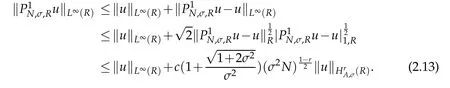
In numerical analysis of Fokker-Planck equations,we need the following estimate on L∞(R)-norm of P1N,σ,Ru.By Proposition 2.2 and Lemma 2.2,we have the following result.

Proposition 2.3.

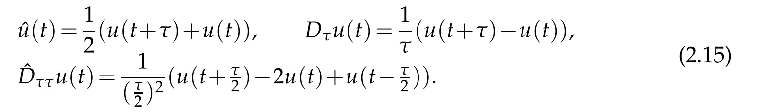
Weneedalemmaintime t-directionfornumerical analysisthefull-discreteofFokker-Planck equations.For this purpose,let[T]be the integer part of any fixed positive constant T,and τ be the mesh size of the variable t.We denote

Let

Lemma 2.3.We have(cf.Lemma 4.6 of[12]),

Remark 2.2.Different from the Section 2 of[30,34],here we work with the problem of variable coefficients by using non-uniformly weighted Sobolev spaces.In equation(1.1),the fact that the power of coefficient of the term?vW(v,t)is even bigger than that of the termW(v,t),brings some difficulties in numerical analysis and actual computation.Moreover,the projectionorthogonal projection defined on the whole line,rather than the composite generalized Laguerre approximation for domain decomposition on the whole line which need to match the numerical solutions on the common boundaries of adjacent subdomains,see[28].

3 Full-discrete scheme for nonlinear Fokker-Planck equations

In this section,we propose the Hermite spectral scheme for the nonlinear Fokker-Planck equations on the whole line,with the convergence analysis.

3.1 Discrete scheme and error analysis

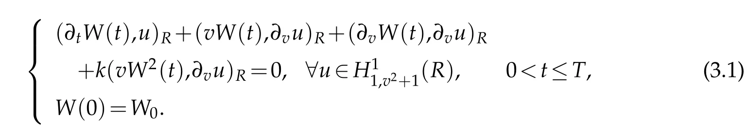
A weak formulation of(1.1)is to seek solutionsuch that

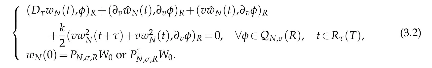
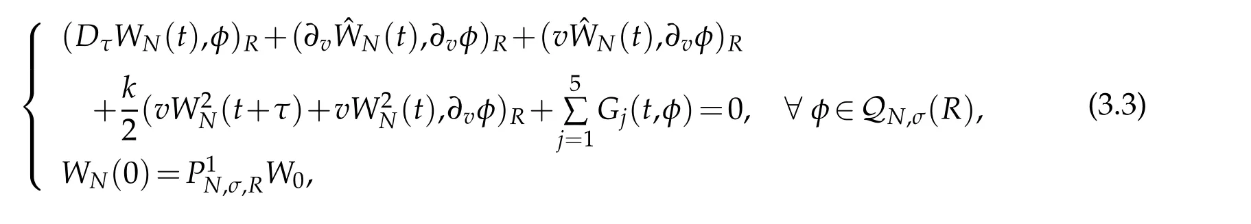
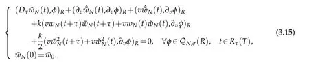
In designing the relevant fully discrete scheme for(3.1),we use Crank-Nicolson scheme in time direction with the mesh size τ.It is to find wN(t)∈QN,σ(R)for all t∈ˉRτ(T)such that

We now deal with the convergence of scheme(3.2).The origin of difficulty in dealing with(3.2)numerically is two order difference terms of nonlinear vW(v,t)(1+kW(v,t)).To estimate the errors caused by the nonlinear terms,letW.By the definition ofττu(t)in(2.15),we have(cf.[34])

In order to analyse numerical errors,we can write

where

We derive the following equation from(3.1)that for t∈Rτ(T)

where

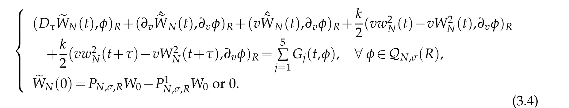
where

Next,we give the main result of our work in this subsection.

Theorem 3.1.andIfwith r≥1,then for all t∈(T),

where b1,b2and b3are positive constants depending on σ and the norms of W in the spaces mentioned above.

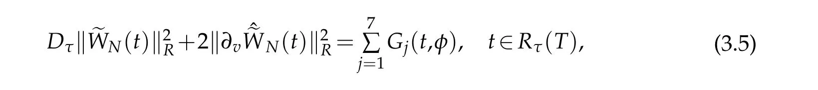
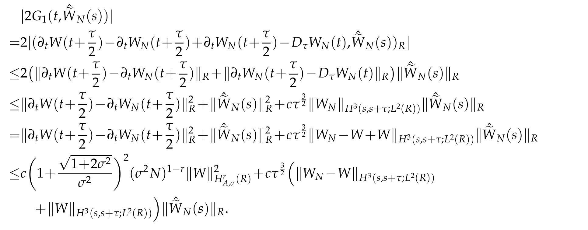
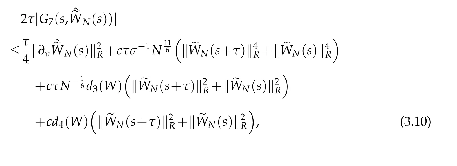
Proof.We estimate the terms|Gj(t,N(t))|in(3.5),1≤j≤7.Let Rτ(t?τ)like Rτ(T)in(2.14).We use Cauchy-Schwarz inequality,Proposition 2.2 with r=1 and Lemma 2.3 to verify that for s∈Rτ(t?τ),

We have

We use Cauchy-Schwarz inequality again and Proposition 2.2,Lemma 2.3 to show that

whence

Now,we are in a position of estimating the Gj(t,φ),j=4,5.By virtue of Proposition 2.2,Lemma 2.2 and(2.13)with r=1,we get that

From the Taylor formula and Lemmas 2.2,Proposition 2.1 withμ=r=0 and(2.11)with r=1,we also have for τ1∈(s,s+)and τ2∈(s+,s+τ)that

A combination of the above estimate gives that

where d1(W)is a certain positive constant depending only on ‖W‖C(s,s+τ;H1A,σ(R)),and d2(W)is a certain positive constant depending only on ‖W‖C1(s,s+τ;H1A,σ(R)).

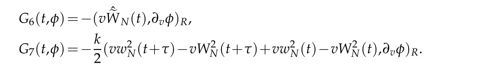
Finally,we estimate Gj(s,φ),j=6,7.A direct result

can be got.By the H¨older’s inequality,Remark 2.1,Lemma 2.1 and Proposition 2.2,we deduce that

Thus,we obtain that

where d3(W)is a certain positive constant depending only ond4(W)is a certain positive constant depending only on ‖vW‖L∞(R).

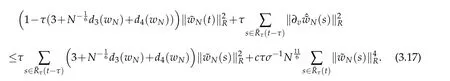
Furthermore,we use(2.10)and(2.11),Proposition 2.1 withμ=0 to derive that

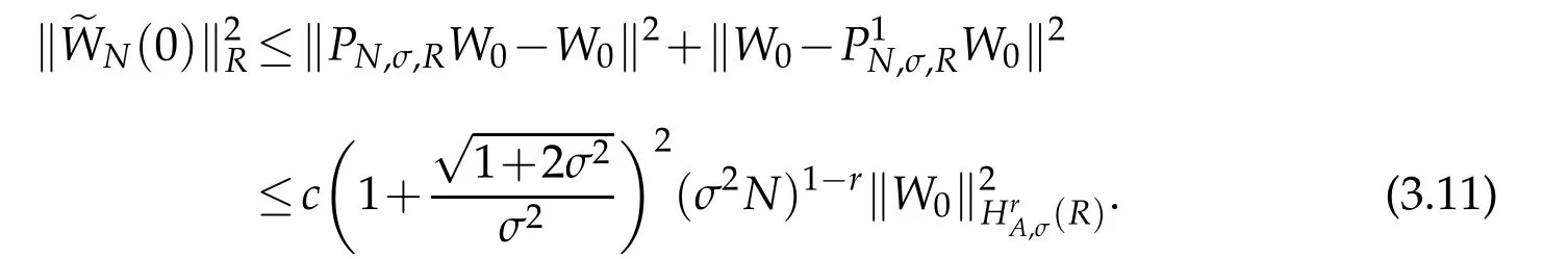
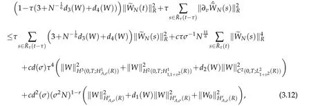
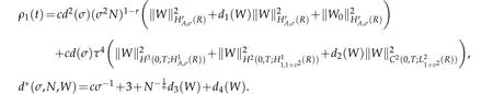
provided ρ1(t)is finite.By Gronwall lemma(see Lemma 3.2 of[12]),we get that

A combination of the above estimate with(2.11)derive the desired result(3.14).

Remark 3.1.The constants d1(W),d2(W)and d3(W)may dependon N whenusing(2.11)with r6=1.

3.2 Stability analysis

We now consider the generalized stability of(3.2).Let?W0be the errors of W0,which induce the error of wN,say?wN.From(3.2),we get that

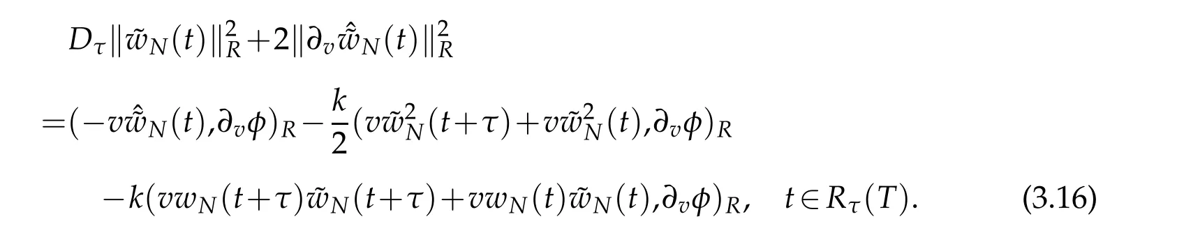
Using the same manner as in derivation of(3.12),we derive that

Let E(u,t)be thesame as in(3.14)andByGronwall lemma(seeLemma3.2 of[12])again,we have the following result that for suitably small τ and certainRτ(T).

Proposition 3.1.then for all t∈ˉRτ(ξ),

where b4and b5are positive constants dependent only onand σ.

4 Numerical results

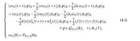
Inthis section,we describe the implementations for the spectralschemes(3.2)witha nonhomogeneousterm f(v,t),and present some numerical results confirming the theoretical analysis.For fixedness,we suppose that k=1 in(3.2)in the forthcoming discussions.We use the Crank-Nicolson discretization in time t,with the mesh size τ.At each time step,we then need to solve a nonlinear equation

In actual computation,we expand the numerical solution as

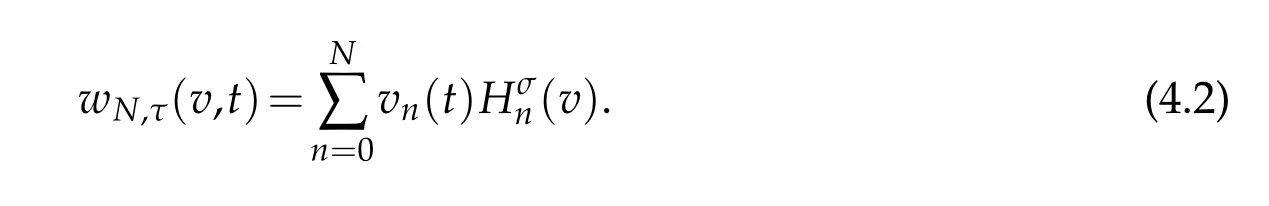
Let

and define the vectors

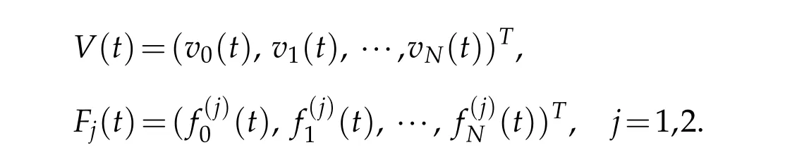
Inserting the above expansion into(4.1)and taking φ=Hσm(v)respectively,in(4.1)for 0≤m≤N,we find that(4.1)is equivalent to the following system of

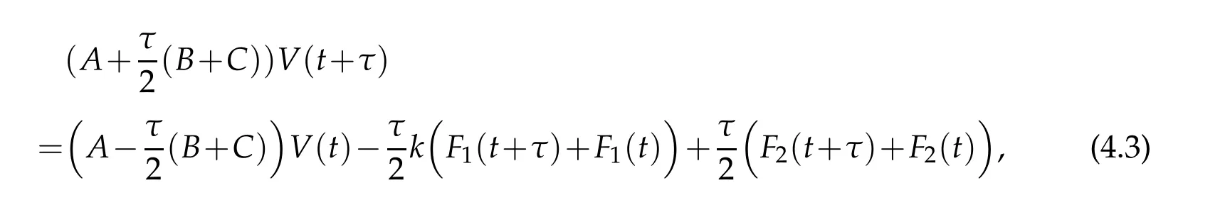
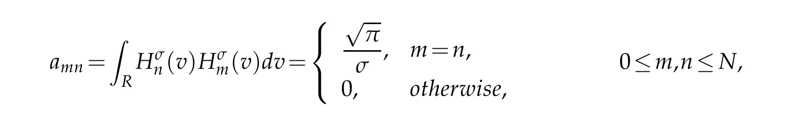
where the matrices A=(amn),B=(bmn)and C=(cmn)have the entries

and

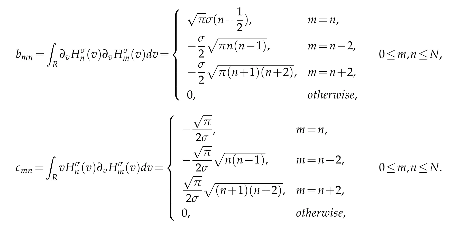
By the orthogonal property of generalized Hermite polynomial,all matrices in(4.3)are some diagonal matrices,pentadiagonal symmetric matrices and pentadiagonal antisymmetric matrices.This feature simplifies the calculation.

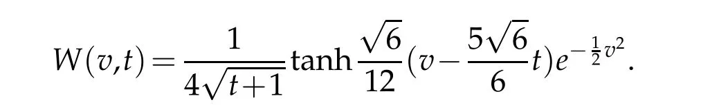
Now,we take the test function

For description of the errorW?wN,Let vN,R,nand ωN,R,nbe the nodes and the weights of the standard Hermite-Gauss interpolation.According to definition(2.1),we can get the nodes and weights of the scaled Hermite-Gauss function interpolation as follows

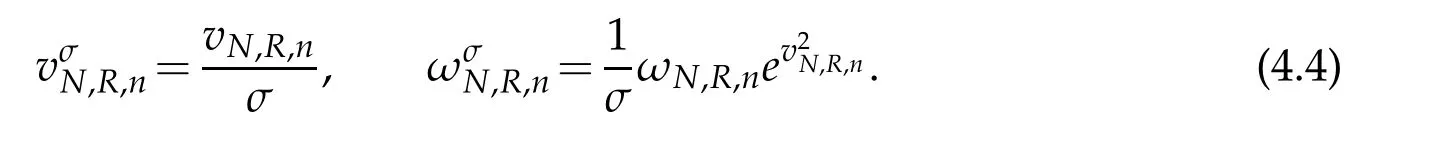
We notate

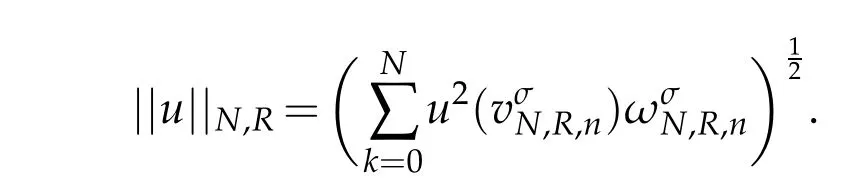
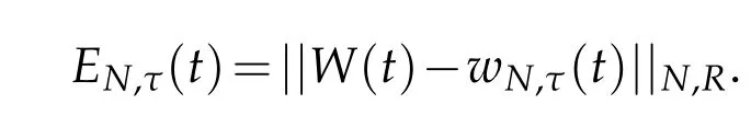
The numerical errors are measured by the discrete norm

In Figure 1,we plot the errors log10EN,τ(t)with t=1 and σ =1.Clearly,the errors decay fast when N increase and τ decreases.The facts coincide very well with theoretical analysis in Section 3.Inparticular,theyshowthe spectral accuracy in the space of scheme(3.2).

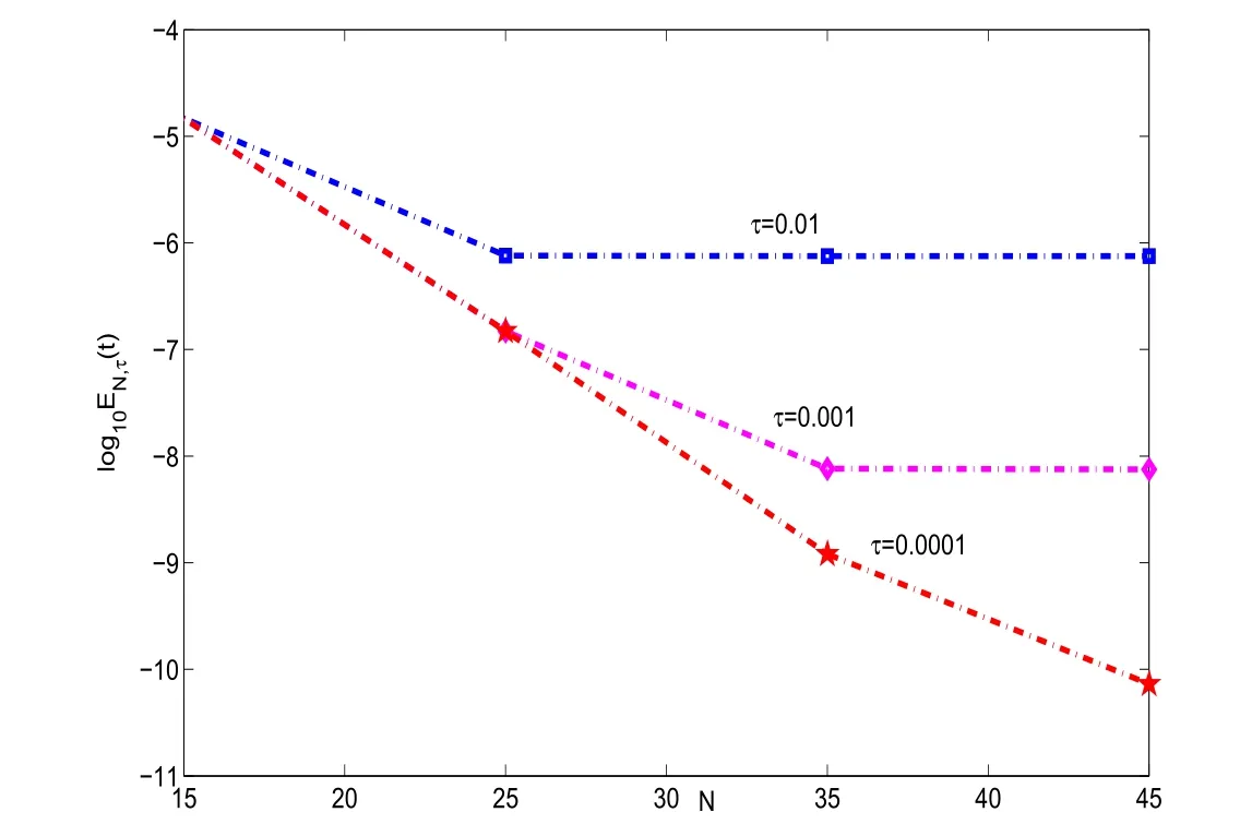
Figure 1:log10EN,τ(1)vs of scheme(3.2)with σ =1 and diあerent τ.

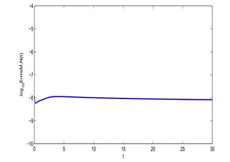
Figure 2:log10EN,τ(t)vs t of scheme(3.2)with τ =0.001,N=36 and σ =1.

In Figure 2,we plot the numerical errors log10EN,τ(t)with σ=1,N=36,τ=0.001,They indicate the stability of scheme(3.2)for long time computing.

For the verification of the validity of the method,we think more forcible numerical examples with solutions having decays algebraically at infinity.To do this,we take the following test function

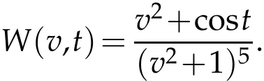
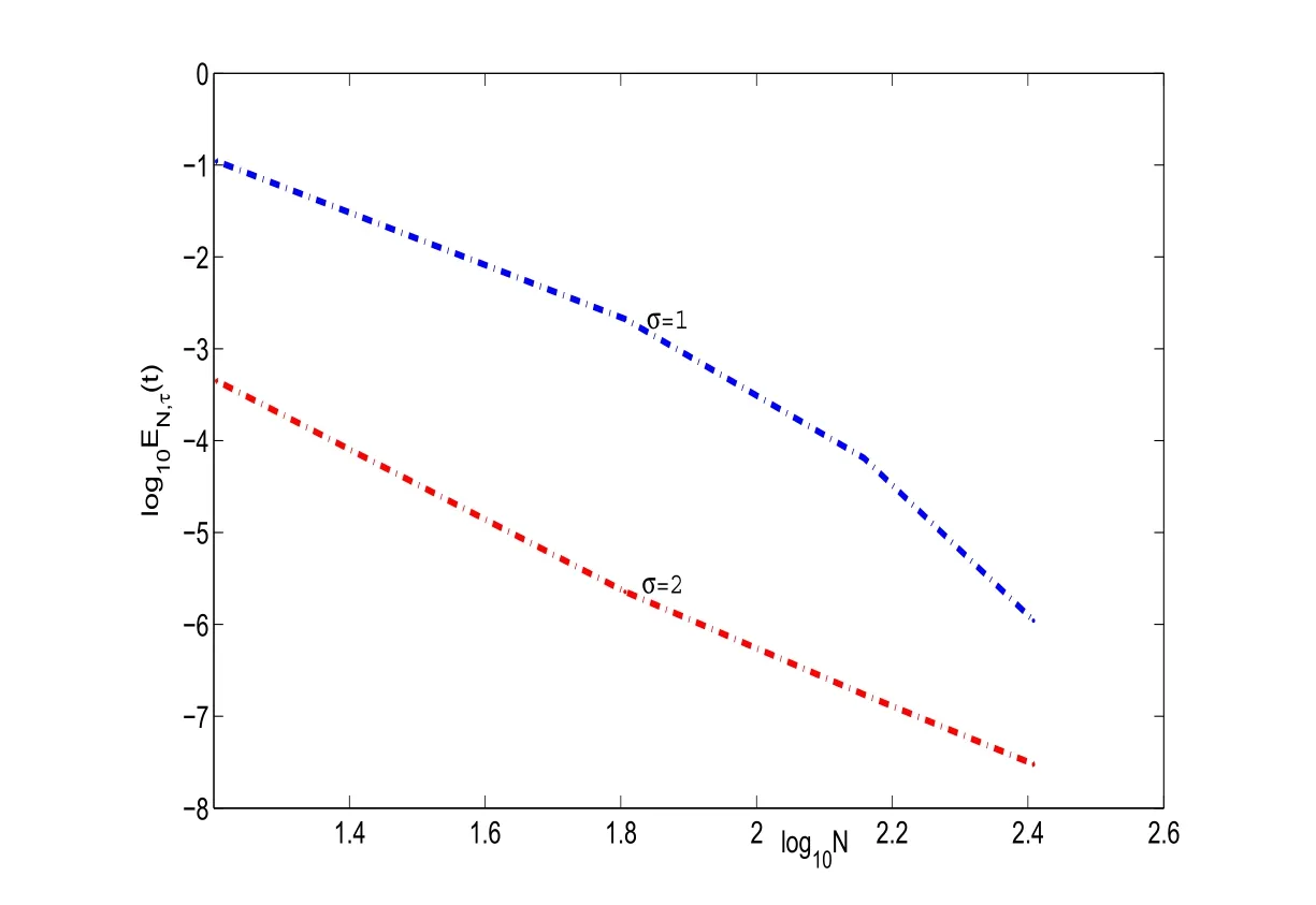
Figure 3:log10EN,τ(t)vs log10N of scheme(3.2)with τ =0.001,and diあerent σ.

In Figure 3,we plot the errors log10EN,τ(t)with t=1 and τ =0.001.Clearly,the errors decay at a certain algebraic rate.We also note that for the same N and τ,the errors for parameter σ =2 in scheme(3.2)are better than that for σ =1 in scheme(3.2).They show the scheme(3.2)is also valid for the solution of(3.1)with decays algebraically at infinity.

5 Concluding remarks

In this paper,we studied numerical simulation of nonlinear Fokker-Planck equations on the whole line,which plays an important role in many fields.We constructed a spectral scheme using the generalized Hermite functions which are orthogonal with weight χ(v)≡1,simplified the algorithm schemes and saved a lot of work.We proved the convergence and stability of the proposed schemes using the approximation of a nonstandard generalized Hermite functions.The numerical results demonstrated the spectral accuracy in space,and coincide well with the theoretical analysis.

The main advantages of the proposed approach are as follows:

?With the aid of the generalized Hermite approximations,we could deal with PDEs properly,and approximate partial differential equations directly.

?By using the generalized Hermite approximations,we could properly deal with the singularities of coefficients v appearing in the underlying differential equations,which varies from?∞to∞.Consequently,we could deal with the problems on the whole domain properly.

? The adjustable parameter σ involved in the generalized Hermite approximation enables us to fit the asymptotic behaviors of exact solutions at infinity closely.

AlthoughweonlyconsideredthenonlinearFokker-Planckequationofone-dimensional,the main idea and techniques developed in this paper are also applicable to many other partial differential equations defined on unbounded domains.

6Acknowledgement

The first author of this work was supported in part by NSF of China No.11401380.The second author was supported in part by NSF of China No.11371123,No.11571151 and No.11771299.