
STABILITY OF RAREFACTION WAVE FOR A MACROSCOPIC MODEL DERIVED FROM THE VLASOV-MAXWELL-BOLTZMANN SYSTEM?
2018-07-23 08:42:00YongtingHUANG黃詠婷
關(guān)鍵詞:紅霞
Yongting HUANG(黃詠婷)
Department of Mathematics,City University of Hong Kong,Hong Kong,China
E-mail:ythuang7-c@my.cityu.edu.hk
Hongxia LIU(劉紅霞)
Department of Mathematics,Jinan University,Guangzhou 510632,China
E-mail:hongxia-liu@163.net
Abstract In this article,we are concerned with the nonlinear stability of the rarefaction wave for a one-dimensional macroscopic model derived from the Vlasov-Maxwell-Boltzmann system.The result shows that the large-time behavior of the solutions coincides with the one for both the Navier-Stokes-Poisson system and the Navier-Stokes system.Both the timedecay property of the rarefaction wave pro file and the influence of the electromagnetic field play a key role in the analysis.
Key words Vlasov-Maxwell-Boltzmann system;rarefaction wave;energy method
1 Introduction
As a fundamental model in plasma physics,the Vlasov-Maxwell-Boltzmann(VMB)system describes the time evolution of dilute charged particles(for example,electrons and ions)under the influence of binary collisions and their self-induced Lorentz forces governed by Maxwell equations,cf.[4],taking the form of


where S2is the unit sphere of R3.The velocity pairs(v,v?)before collisions andafter collisions are defined by

in terms of the conservation of momentum and kinetic energy

The collision kernel q(v ? v?,ω) ≥ 0 depends only on the relative velocity|v ? v?|and the deviation angle ? given byThroughout this article,we assume that q(v ?v?,ω)is determined by the collision between particles with hard-sphere interaction in the form of

For more physical situations,for instance,we expect that the techniques developed in this article together with the ones in[36]can be applied to the soft potential case.
The VMB system was intensively studied and many important progress were made.On the perturbation theory,Guo[17] first established the global-in-time existence of classical solutions around the global Maxwellian equilibrium state in three-dimension torus and the corresponding existence result in the whole space was proved by Strain[35].The diffusive limits of the VMB system in a periodic box was constructed by Jang[22].The local stability and large-time behavior of solutions to the Cauchy problem in R3are studied by Duan-Strain[14],Duan-Liu-Yang-Zhao[7]and many references therein.Recently,Li-Yang-Zhong[26]and Huang[21]studied the spectrum structures of the VMB system with and without angular cutoff assumption respectively while the optimal convergence rates of the solutions are obtained as the application.We would point out that the self-consistent electromagnetic field makes the dissipative structure of the VMB system(1.1)more complicated than both the classical Boltzmann equation and the closely related Vlaso-Poisson-Boltzmann(VPB)system.
To the best of our knowledge,so far there have been few mathematical results clarifying the asymptotic behavior of solutions of the VMB system tending to a rarefaction wave.In the content of Boltzmann equation without any force,whenever the initial data tend to distinct global Maxwellians at far fields,instead of converging to a constant equilibrium,the solution to the Cauchy problem usually approaches time-asymptotically towards the wave patterns of the Boltzmann equation.The studies on stability of basic wave patterns for Boltzmann equation are rather satisfactory.Ca filisch-Nicolaenko[1]proved the existence of the Boltzmann shock pro files.The stability and optimal convergence rate of the shock pro file are studied by Liu-Yu[31]and Yu[39].Liu-Yang-Yu-Zhao[30]and Xin-Yang-Yu[36]proved the nonlinear stability of rarefaction waves for the Bolzmann equation.Huang-Yang[20]and Huang-Xin-Yang[19]showed the stability of contact discontinuities both with and without zero mass condition.As far as the rarefaction wave of the Boltzmann equation is concerned,the pro file is in the form of a local Maxwellian associated with the macriscopic quantities formally determined by the conservation laws,where initial data are given by far- field global Maxwellians.The approach to study the local stability of such local Maxwellian is mainly based on the energy method proposed by Liu-Yu[31],developed by Liu-Yang-Yu[29],with further improvement in Yang-Zhao[37].When the electric field is included,as it has already been studied in Duan-Liu[10,12],Li-Wang-Yang-Zhong[25]and so on about the rarefaction waves of the VPB system,the dissipative property of the Poisson equation contributes a lot to the analysis.Back to the fluid level,Duan-Yang[8],Duan-Liu[11],and Duan-Liu-Yin-Zhu[13]proved the stability of the rarefaction wave of the Navier-Stokes-Poisson(NSP)system.Motivated by[11,12,23,25,27,28,33,38],we consider the stability of the rarefaction wave for a one-dimensional macroscopic model derived from the VMB system(1.1)in this article.The current analysis could provide a clue to hopefully derive the time-asymptotic behavior of the rarefaction wave of the Navier-Stokes-Maxwell system and the VMB system.
In one-dimensional space,without any ambiguity we use x to denote x1∈R and the macroscopic model derived from the VMB system(1.1)takes the form of

where the fluid quantity n=n(t,x)such that n=?xE1satisfies

The details of the derivation of equations(1.2)will be given in the Appendix.The macroscopic model(1.2)forms a closed system of conservation equations containing eight unknowns:the density ρ = ρ(t,x)>0,the velocity u=(u1,u2,u3)=(u1,u2,u3)(t,x),the temperature θ= θ(t,x)>0,the electric field E=(E1,E2,0)=(E1,E2,0)(t,x),and the magnetic field B=(0,0,B3)=(0,0,B3)(t,x)for t≥0,x∈R.P denotes the pressure function satisfyingThe coefficients μ(θ),κ(θ),κ(θ)are all positive smooth functions depending only on θ.Here and in the sequel,for simplicity,we denote E+u×B=(E1+u2B3,E2?u1B3,0).
Initial data of system(1.2)are given by

with far- field states

where ρ±,θ±>0,and u±=(u1,±,0,0)are assumed to be constant states.The boundary values of the electromagnetic field at infinity are set by

We are interested in studying the large-time behavior of solutions to the Cauchy problem(1.2)under the conditions(1.4)–(1.6)in the case
Recall that the one-dimensional NSP system takes the form,cf.[6,13],

where for ν =i,e,qi=1 and qe= ?1 are the charges of ions and electrons.ρν= ρν(t,x)>0,,and θν= θν(t,x)>0 are the density,velocity,and temperature of ν- fluid.The pressure Pν=Rρνθνwith R>0 being the gas constant.E1=E1(t,x)∈ R is the electric field.The constantsμν,κν>0 denote the viscosity and heat conduction coefficients.Consider the conservation equation for ρi? ρeof system(1.7)for a special case:=ui=ue,

We would like to mention that equation(1.3)is derived from taking the difference between the two governing equations(1.1)1and(1.1)2.Without the influence of the magnetic field,that is,E2=B3=0,equation(1.3)is reduced to

It holds true that some techniques for the NSP system(1.7)can be applied to the reduced system for(1.2).
We establish the global-in-time asymptotic stability of the rarefaction wave for the system(1.2)under the smallness assumption on the perturbation while additional smallness assumption on the initial boundary data and the wave strength is imposed because of the influence of the magnetic field.The main result in Theorem 2.1 shows that the large-time behavior of solutions coincides with the one for both the NSP system and the Navier-Stokes system because the asymptotic pro file of the electromagnetic field is assumed to be trivial.The proof is based on the classical energy method.Compared to the analysis for NSP system,additional difficulties occur because of the appearance of the magnetic field,which can be overcome by the combination of the techniques employed in[11]with delicate dissipative properties of system(1.2).
The rest of this article is arranged as follows.In Section 2,we construct a smooth approximation of the rarefaction wave and the nonlinear stability of the rarefaction wave is given.The proof of the a priori estimates is sketched in Section 3 and the proof of the main result Theorem 2.1 is concluded in Section 4.In the Appendix,we provide a derivation of our macroscopic model(1.2)from the VMB system(1.1).
NotationsThroughout this article,? denotes some generic small positive constant,which may take different values in different places.means that there is a generic constant C>0 such thatstands for the Lp(Rx)-norm.For convenience,we use k·k to denote the L2(Rx)-norm and Hk(Rx),k≥0,to denote the usual Sobolev space with respect to x variable.
2 Asymptotics Toward the Rarefaction Wave
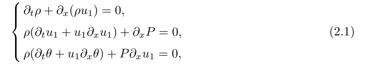
In this section,we study the asymptotic stability of the rarefaction wave for the Cauchy problem(1.2)and(1.4)–(1.6)of the one-dimensional macroscopic model derived from the VMB system(1.1).We expect that(ρ,u1,θ)(t,x)tends time-asymptotically towhich is defined to be the centered rarefaction wave solution to the the Riemann problem on the compressible Euler system
with Riemann initial data given by

2.1 Approximate rarefaction wave
The thermodynamic law

where S denotes the entropy,v is the specific volume,that is,v=1/ρ,implies

for some constant k>0.So the pressure can be rewritten as

It is equivalent to consider the Euler system(2.1)in terms of(ρ,u1,S),cf.[34],


with corresponding right eigenvectors ri=ri(ρ,u1,S),i=1,2,3,

The three pairs of Riemann invariants associated with these eigenvectors can be taken as


Here and in the sequel,S?is a constant such that

In what follows,we construct a smooth approximation of the rarefaction wave corresponding to the solution to the Riemann problem(2.1)–(2.2).Consider the Riemann problem on the Burgers’equation

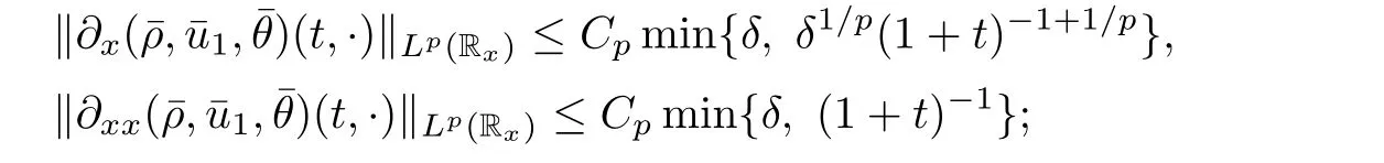
for w? The solution to the Burgers’equation becomes smooth when the initial data is replaced by some smooth increasing function.That is,for given constants w? which holds the following basic properties. Lemma 2.1([32],Lemma 2.1)Suppose w+>w?and setThe Cauchy problem(2.8)admits a unique smooth global solution satisfying (ii)For any p∈[1,∞],there exists a constant Cpsuch that for t≥0, (iii) In fact,the i-th rarefaction wave can be constructed along the given curve Riwhenever the i-th characteristic λi= λi(ρ,u1,S)satisfies the Burgers’equation with increasing data,i=1,3.Without loss of generality,here we consider the 3-rarefaction wave and the 1-rarefaction wave can be treated similarly.Forthe Riemann problem(2.1)–(2.2)admits a self-similar solution,the 3-rarefaction wave(x/t),explicitly given by In order to justify the large-time behavior of the solution(ρ,u1,θ)(t,x)to the pro file(x/t),we usually deal with the stability analysis of its smooth approximationin the framework of small perturbation.Corresponding to(2.9),the smooth rarefaction wavecan be defined by Lemma 2.2Letbe the wave strength.The approximate rarefaction pro filedefined by(2.8)and(2.10)satisfies (ii)For any p∈[1,∞],there exists a constant Cpsuch that for t≥0, (iii) ProofRecall(2.4)and(2.10),it holds that which follows and In this subsection,we study the stability of the approximate rarefaction waveof system(2.11)for the Cauchy problem(1.2)and(1.4)–(1.6).We define the perturbation which satisfies the following system, Notice that ψ =(ψ1,u2,u3)and initial data of the above system are given by The main result of this article is stated as follows. Theorem 2.1Consider the Cauchy problem of the one-dimensional macroscopic system(1.2)derived from the VMB system(1.1)supplemented with the conditions(1.4)–(1.6).Assumewhereis given in(2.6)with ρ?,θ?>0.Let δ=|ρ+? ρ?|+|u1+? u1?|+|θ+? θ?|be the wave strength.There are small constants ε0, ε1>0 such that if while the far- field states and the wave strength are additional supposed to satisfy then the Cauchy problem(2.14)–(2.15)admits a unique global solution(φ,ψ,ζ,E1,E2,B3)(t,x)satisfying Moreover,the solution to the original Cauchy problem(1.2)and(1.4)–(1.6)tends time-asymptotically to the rarefaction in the sense that Remark 2.1The proof is based on the classical energy method.Additional smallness assumption on the initial boundary data and the wave strength(2.17)is imposed because of the appearance of the magnetic field.Precisely,the smallness of the pro fileis essential to prove the a priori estimate such that by(2.10)and(2.17),it holds that When investigating the stability of the rarefaction waves of the NSP system and the VPB system,the Riemann problem on the corresponding Euler system admits a rarefaction wave whose strength is not necessarily small,cf.[8,10–12]. Remark 2.3Inspired by[10,12]and[25],we expect to study the existence and stability of nontrivial large time asymptotic pro files for the one-dimensional VMB system(5.26)with slab symmetry.The main difficulty in the analysis is the lack of estimates for highest-order spatial derivatives of the electromagnetic field,which is a typical feature of the VMB system with regularity-loss property.Precisely,trouble occurs in the highest-order weighted energy estimates onFor|α|=2,it holds that Here,for t>0,x1∈ R,v ∈ R3,M±are defined in(5.14)andis a global Maxwellian such that the constant states(ρ?,u?,θ?)with u?=(u1?,0,0)satisfying for some η0>0 suitably small,cf.[25].In one-dimensional space,the large-time behavior of F±has a slow time-decay rate and such a term is not time-space integrable.So far,the stability of the rarefaction wave for the one-dimensional VMB system is open. To deduce the a priori energy estimates on the fluid quantities(φ,ψ,ζ,n)and the electromagnetic field(E,B),we do the following a priori assumption, where and in the sequel χ is a small positive constant depending on the initial data and wave strengths.Following the Sobolev’s inequality, we can deduce from the a priori bound(3.1)that The desired energy type estimates are based on the a priori assumption(3.1),the estimates onin Lemma 2.2 with the additional condition(2.17)on the initial far- field states and the wave strength. Step 1Zero-order energy estimate. Firstly,we define the following entropy functional where Notice that as|(φ,ζ)|can be suitably small.Hence,the functional η(t,x)is equivalent to|(φ,ψ,ζ)|2.Multiplying(1.2)1byit holds that By(1.2)1,(2.11)1,and(2.11)3,direct calculations yield that which lead to where It follows from(1.2)5that Multiplying(2.14)i+1by ρψi,i=1,2,3,the summation of the resulting equations yields The summation of(3.4)+3/2{(3.5)+(3.6)}leads to Then,we consider the zero-order energy estimate of the electromagnetic field.Multiplying(2.14)6by E1,and recalling n=?xE1,it holds that The technical part to treat equation(3.8)comes from the termon the right-hand side.As u2=ψ2,we rewrite this term as to make use of the dissipation of E+u×B and the positive weightMultiplying(2.14)7byand(2.14)8by B3,the summation of the two obtained equalities leads to As using(3.9),we combine(3.8)and(3.10)to obtain Taking the summation of(3.7)+3/2(3.11),we arrive at the following equality, where we used the identity for some positive constant c.To prove(3.13),recalling(2.13),we rewrite H5as the statement follows from the direct calculations under the a priori assumption(3.1).On the other hand,we use(2.21)to obtain Hence,the integration of(3.12)with respect to x,τ over R×[0,t]leads to Before further estimates on the right-hand terms of the above inequality,by Lemma 2.2,we deduce some estimates on the pro fileWe claim that for 0<δ≤1 and any α∈(0,1),especially for α≤1/4,we have The terms Ii,i=1,···,8,of(3.14)are estimated as follows.Firstly,we do integration by parts,using H?lder’s inequality,Sobolev’s inequality(3.2),(3.15),Lemma 2.2 and Young’s inequality,to obtain Similarly,we can claim that Recalling(2.11),it is obtained from H?lder’s inequality,(3.16),and the a priori assumption(3.1)that And it follows from the Cauchy-Schwarz inequality that where we used Lemma 2.2 and the a priori assumption(3.1)to obtain Under condition(2.21),we can claim Finally,from H?lder’s inequality,the a priori assumption(3.1),and Lemma 2.2,we obtain the followings: Substituting the above estimates for Ii,i=1,···,8,into(3.14),for δ,χ being suitably small,it holds that Step 2The dissipation of?xφ. Multiplying(2.14)2by ?xφ,it holds that where we used(2.14)1to obtain Differentiate(2.14)1with respect to x,we have where we used identity(1.2)1to obtain Integrating{(3.18)+(3.20)}with respect to x,τ over R×[0,t],it holds that Firstly,it is direct to obtain the following: Then,we use(3.16)to claim that and As for I17,it follows that where and we used(3.16)again to claim that Similarly,we can claim Substituting the above estimates for Ii,i=9,···,20,into(3.18),for δ,χ being suitably small,it holds that Step 3The dissipation of(n,?xn). Multiplying(1.3)by n,and recalling n= ?xE1and u2= ψ2,it yields that The integration of(3.23)with respect to x,t over R×[0,t]leads to Here, Similarly,we have Finally, Then,we can claim that The combination of{(3.17)+(3.24)+ κ1(3.22)}for κ1>0, δ,χ >0 being suitably small yields that Using Gronwall’s inequality,it follows from(3.25)that Step 1The dissipation of?xx(ψ,ζ). Applying?xto equation(2.14)i,i=2,3,4,5,we have and Notice that Integrating(3.29)with respect to x,τ over R×[0,t],it holds that We now turn to estimate Ji,i=1,2,···12,term by term.For the sake of brevity,we give straightforward calculations as follows: and It remains to estimate the terms coupling with the electromagnetic field.It is directly to see Substituting the above estimates for Ji,i=1,···,12,into(3.30),we arrive at Step 2The dissipation of?x(E2,B3). Differentiate(2.14)i,i=7,8,with respect to x and multiply the resulting identities by?xE2and ?xB3,respectively.The summation of the two equations yields that Integrating(3.32)with respect to x,τ over R×[0,t],it holds that where And we use(2.21)again to obtain Substituting the above estimates into(3.33),we can claim It remains to estimate ?xB3.Multiplying(2.14)7by ?xB3,and replacing ?tB3by ??xE2,we have The integration of the above equality with respect to x,τ over R×[0,t]yields Taking a combination of(3.31)+(3.34)+ κ2(3.36)for κ2>0, δ,χ >0 being sufficiently small,we can claim the higher order estimate as below, The local existence of the solution(φ,ψ,ζ,E1,E2,B3)(t,x)of the reformulated Cauchy system(2.14)–(2.15)can be obtained by the standard iteration methods,cf.[5,18].To prove Theorem 2.1,it is sufficient to show the following global-in-time a priori estimates. Proposition 4.1Suppose that all assumptions in Theorem 2.1 hold.If the solution to the Cauchy problem(2.14)–(2.15)on 0 ≤ t≤ T for T>0 satisfies for some constants ε0>0 being sufficiently small,and additional smallness assumption(2.17)holds,then we can claim that ProofTaking a suitable combination of(3.26)+κ3(3.37)for some κ3>0 suitably small,we arrive at As?xE1=n,(4.1)follows.? We end up this section with the proof of Theorem 2.1. Proof of Theorem 2.1The existence of the solutions follows from the standard continuity argument based on the local existence and the a priori estimate in Proposition 4.1.Therefore,it suffices to show the large time behavior of the solutions.We first claim the estimates and Indeed,by(3.20),(3.29),(2.18),and Lemma 2.2,we can show that Following from the above inequality and(2.18),it holds that which implies(4.3).Secondly,from(3.23),(3.32),(2.18),and Lemma 2.2,we obtain Similarly,(4.4)follows from the above inequality and(2.18). From(4.3),(4.4),and the Sobolev’s inequality(3.2),we consequently obtain and Furthermore,by the construction of the smooth approximation of the rarefaction wave,in terms of(iii)in Lemma 2.2,we obtain the desired asymptotic behavior of the solution In this section,we provide a derivation of the one-dimensional macroscopic model(1.2)from the VMB system(1.1).It is mainly based on the macro-micro decompositions of the Boltzmann equation,cf.[29].With some cancellation property in the original system,set system(1.1)can be reformulated as We would point out that in absence of the electromagnetic field,(5.1)1is reduced to the Boltzmann equation.Recall that the Boltzmann collision operator Q(·,·)has five collision invariants ?j= ?j(v),j=0,···,4, such that for any measurable,rapidly decaying functions F=F(·,v), Particularly,it holds that As in[29],in terms of the solution F1(t,x,v)to system(5.1),we introduce the five conserved quantities,the mass density ρ = ρ(t,x),the momentum ρu=(ρu)(t,x),and energy ρ(e+|u|2/2)=(ρ(e+|u|2/2))(t,x)by We construct the local Maxwellianin the form of where θ= θ(t,x)>0 is the temperature related to the internal energy e(t,x)by e=3Rθ/2 with R being the gas constant and u=u(t,x)=(u1,u2,u2)(t,x)is the fluid velocity.With respect to M,we define an inner productin the spaceas for functions F(·,v),G(·,v)such that the integral is well defined.With respect to this inner product,the macroscopic subspace NMspanned by the collision invariants can be constructed by the following orthogonal basis, where δijis the Kronecker delta.The macroscopic projection P0and the microscopic projection P1defined as are orthogonal and thus self-adjoint with respect to the inner product h·,·iM,that is, We decompose F1=F1(t,x,v)of(5.1)into the combination of the local Maxwellian M and the microscopic component G=G(t,x,v)as The microscopic equation for G is obtained by applying the microscopic projection P1to(5.1)1, where LMis the linearized collision operator given by It is seen that the null space of LMis exactly NMand LMis a bounded and one-to-one operator onIt follows from(5.6)that where Recalling(5.3),for F2=F2(t,x,v)governed by(5.1)2,there is only one conserved quantity n=n(t,x)defined by As in[25],we introduce another macro-micro projections around the local Maxwellian M such that The macroscopic projection Pdand microscopic projection Pcare also self-adjoint with respect to the inner product h·,·iM.F2(t,x,v)can be decomposed into To obtain the microscopic equation for PcF2=PcF2(t,x,v),we use(5.9)to rewritten equation(5.1)2as The bounded linear operator NM,given by which further implies with Before further discussion,we give a remark on the macro-micro decompositions for F±(t,x,v)of the original system(1.1). Remark 5.1Let F±=F±(t,x,v)be functions satisfying the VMB system(1.1).We decompose F±respectively as,cf.[12], The local bi-Maxwellians involve six macroscopic quantities determined by Therefore,M±is well defined and G±(t,x,v):=F±?M±denote the microscopic parts. On the basis of decompositions(5.5)and(5.9),equations(5.1)1–(5.1)2lead to coupled systems containing the conservation laws for the macroscopic components(ρ,u,θ,n),taking the form and which follow from properties(5.2)–(5.3).Here,the microscopic components G,PcF2are governed by(5.7)and(5.12),respectively,and P is the pressure for the monatomic gases satisfying the state equation, In the sequel,we normalize the gas constant R to be 2/3 so that e= θ and P=2ρθ/3.Moreover,the governing equations of the electromagnetic field satisfy Recalling(5.7),the viscosity and heat conductivity terms in system(5.15),given by,cf.[4,24], where are independent of the density gradient?xρ with smooth coefficients μ(θ),κ(θ)>0.Similarly,we define some positive smooth function κ(θ),cf.[25],by such that Substituting(5.7)and(5.12)into systems(5.15),(5.16),and(5.17),and using(5.18)and(5.19),it yields the fluid-type system for(ρ,u,θ)such that and the fluid quantity n satisfies The electromagnetic field(E,B)is governed by If all microscopic terms Π1and Π2are set to be zero in system(5.20)–(5.22),then we have a closed viscous fluid-type system of eleven unknowns ρ,u=(u1,u2,u3),θ,E=(E1,E2,E3),B=(B1,B2,B3)as below,cf.[9,12,26], where n= ?x·E satisfies Note that(5.23)could be thought as the first-order fluid dynamic approximation of the VMB system(1.1). In one space dimension and only one momentum dimension case,the Maxwell equations degenerate to the Poisson equation.To retain the hyperbolic structure the VMB system,we consider the so-called one and one-half dimensional model proposed by Glassey-Schaeffer[15].It is known that from equations(1.1)5–(1.1)6,we can claim for some vector potential A=(A1,A2,A3)and scalar potential Φ.For the sake of simplicity,we may assume in our work that the rarefaction wave is linearly polarised in the direction x2.Imposing the Coulomb gauge?·A=0,that is,?x1A1=0,(5.25)becomes,cf.[2,16], Thus,in one dimensional space,the VMB system with slab symmetry takes the form of Here the number density distribution functions F±=F±(t,x1,v)have position x1∈ R and velocity v=(v1,v2,v3)∈R3at time t≥0;E=E(t,x1)=(E1,E2,0)(t,x1)and B=B(t,x1)=(0,0,B3)(t,x1).System(1.2)is derived from the one-dimensional VMB system(5.26)following the same procedure from(1.1)to obtain(5.23)and we omit details for simplicity.


2.2 Stability of the rarefaction wave


3 The a Priori Estimates


3.1 Lower-order energy estimate


3.2 Higher-order energy estimate


4 Global Existence and Large Time Behavior


5 Appendix:Derivation of the Model From the VMB System


 猜你喜歡
小學(xué)生作文(低年級(jí)適用)(2022年6期)2022-06-23 06:06:32新高考·英語(yǔ)基礎(chǔ)(高一)(2022年3期)2022-04-29 05:06:32小學(xué)生作文·小學(xué)低年級(jí)適用(2022年4期)2022-04-27 00:30:40作文周刊·小學(xué)一年級(jí)版(2020年40期)2020-10-19 04:42:20Journal of Acupuncture and Tuina Science(2020年4期)2020-08-29 02:49:54大東方(2018年1期)2018-05-30 01:27:23華南理工大學(xué)學(xué)報(bào)(自然科學(xué)版)(2017年4期)2017-06-19 18:25:50作文周刊·小學(xué)一年級(jí)版(2016年28期)2017-06-03 00:28:49中學(xué)生數(shù)理化·八年級(jí)物理人教版(2015年10期)2016-01-04 08:16:33中國(guó)火炬(2014年7期)2014-07-24 14:21:26
猜你喜歡
小學(xué)生作文(低年級(jí)適用)(2022年6期)2022-06-23 06:06:32新高考·英語(yǔ)基礎(chǔ)(高一)(2022年3期)2022-04-29 05:06:32小學(xué)生作文·小學(xué)低年級(jí)適用(2022年4期)2022-04-27 00:30:40作文周刊·小學(xué)一年級(jí)版(2020年40期)2020-10-19 04:42:20Journal of Acupuncture and Tuina Science(2020年4期)2020-08-29 02:49:54大東方(2018年1期)2018-05-30 01:27:23華南理工大學(xué)學(xué)報(bào)(自然科學(xué)版)(2017年4期)2017-06-19 18:25:50作文周刊·小學(xué)一年級(jí)版(2016年28期)2017-06-03 00:28:49中學(xué)生數(shù)理化·八年級(jí)物理人教版(2015年10期)2016-01-04 08:16:33中國(guó)火炬(2014年7期)2014-07-24 14:21:26
 Acta Mathematica Scientia(English Series)2018年3期