Jiaquan Xie , Fuqiang Zhao Zhibin Yao and Jun Zhang

1 Introduction

The elliptic partial differential equations have been applied in various fields of engineering and science. Many important phenomena in electromagnetics, viscoelasticity, fluid mechanics, electrochemistry, biological population models, signals processing [Arpaci(1984); Arpaci and Roache (1972); Myint-U and Debnath (2007); Spotz and Carey (1996);Wang, Zhong and Zhang (2006); Cebeci (2002)] can be well described by elliptic fractional differential equations. For that reason we need a reliable and efficient technique for the solution of fractional differential equations.

The research of numerical solution is still an important subject. Various numerical methods have been proposed to solve such problems. These methods include meshless methods[Dehghan and Shirzadi (2015); Hu, Li and Cheng (2005)], spline collocation methods[Fairweather, Karageorghis and Maack (2011); Abushama and Bialecki (2008)], finitedifference methods [Britt, Tsynkov and Turkel (2010); Boisvert (1981); Singer and Turkel(2006)], finite element method [Ciarlet (2002)], Chebyshev polynomials method [Ghimire,Tian and Lamichhane (2016)], new wavelet based full-approximation [Shiralashetti, Kantli and Deshi (2016)] and Domain decomposition method [Zhang, Zhang and Yin (2008)]. In Aziz et al. [Aziz and Asif (2017)], the authors utilized Haar collocation method for threedimensional elliptic partial differential equations. R. C. Mittal and S. Dahiya used cubic B-spline differential quadrature method to obtain the numerical solution of three-dimensional telegraphic equation in Mittal et al. [Mittal and Dahiya (2017)]. In Srivastava et al.[Srivastava, Awasthi and Chaurasia (2017)], they proposed the reduced differential transform method to solve two and three-dimensional second order hyperbolic telegraph equations.

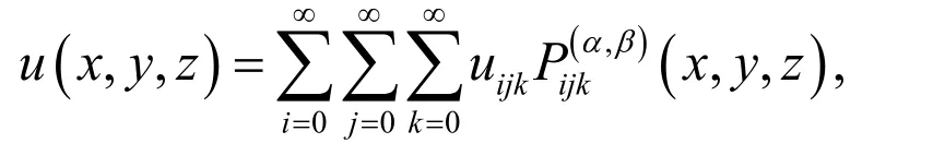
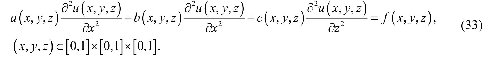
In this paper, we consider the three-dimensional multi-term fractional-order PDEs with variable coefficients of the following form using three-variable shifted Jacobi polynomials:

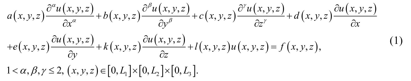
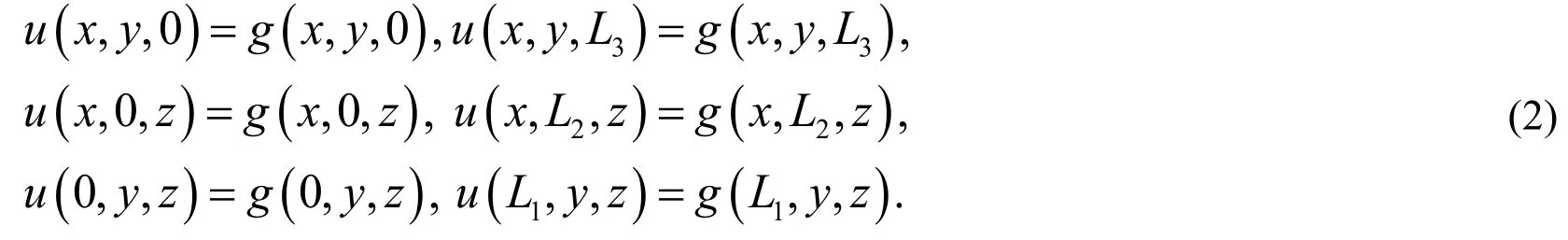
wheredenotes the Caputo derivative,is a known function andis the solution function to be determined. Subject to the Dirichlet boundary conditions:

The current paper is organized as follows: In next Section, the definitions of fractional calculus and shifted Jacobi polynomials, and function approximation are introduced. The differential operational matrix of one-variable shifted Jacobi polynomials is given in Section 3. In Section 4, the error bound and convergence analysis is investigated through some theorems and lemmas. In Section 5, we utilize the three-variable shifted Jacobi polynomials to solve three-dimensional PDEs with variable coefficients. In Section 6,several numerical examples are illustrated to test the proposed method. Finally, a conclusion is drawn in Section 7.

2 Preliminaries and notations

2.1 The fractional derivative in the Caputo sense

Definition 1. The Riemann-Liouville fractional integral operator of orderis defined as [Zhao, Huang, Xie et al. (2017)]

Definition 2. The Caputo fractional derivatives of orderv is defined as Zhao et al. [Zhao,Huang, Xie et al. (2017)]

whereis the classical differential operator of orderm .For the Caputo derivative we have

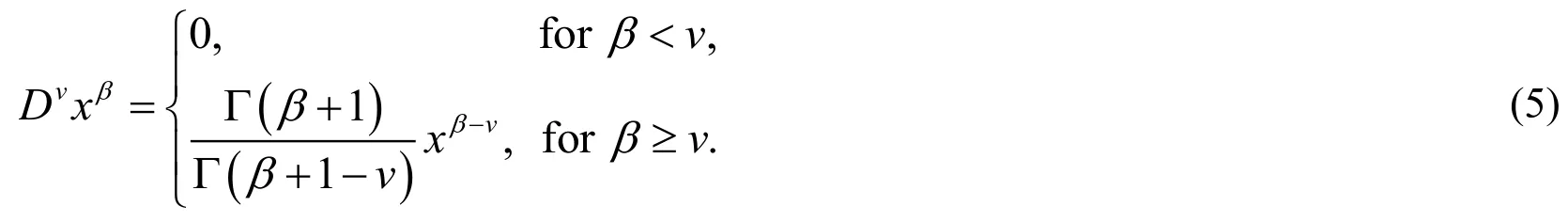
Recall that forv∈N , the Caputo differential operator coincides with the usual differential operator of an integer order.

Similar to the integer-order differentiation, the Caputo’s fractional differentiation is a linear operation, i.e.

where λand μare constants.

2.2 Jacobi polynomials

The well-known Jacobi polynomials are defined on the interval [-1, 1] and can be generated with the aid of the following recurrence formula [Bhrawy and Zaky (2015)]:

whereand

In order to use these polynomials on the intervalwe define the so-called shifted Jacobi polynomials by introducing the change of variable. Let the shifted Jacobi polynomialsbe denoted byThencan be generated from：

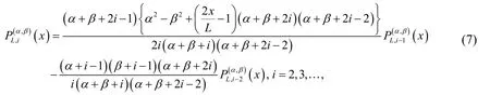
whereand

The analytical form of the shifted Jacobi polynomials

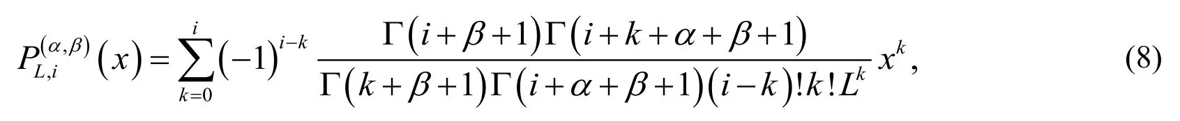
where

The orthogonality condition of shifted Jacobi polynomials is

where

Definition 3. Suppose thatis the sequence of one-variable shifted Jacobi polynomials on the interval. Three-variable Jacobi polynomials,are defined on the domainas follows:

Theorem 1. The polynomialsare orthogonal with respect to the weight function

On the hand, the following property is held:of degreei is given by

Lemma 1. Ifandare jth and kth shifted Jacobi polynomials,the product ofandare written as

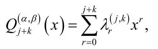
where coefficientare determined as follows:

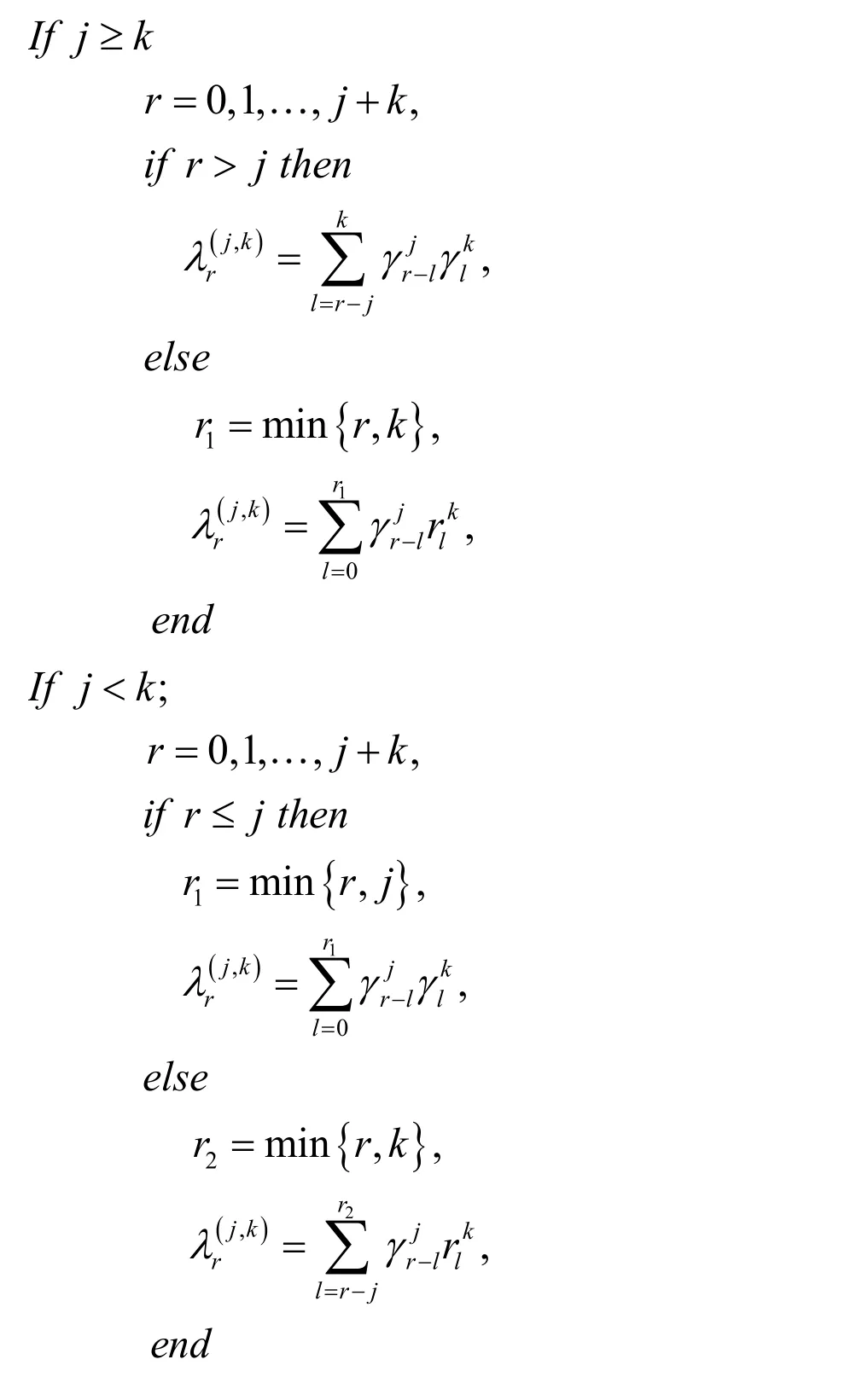
Proof. See Borhanifar et al. [Borhanifar and Sadri (2015)].

Lemma 2. Ifandarei, j andkth shifted Jacobi polynomial,then

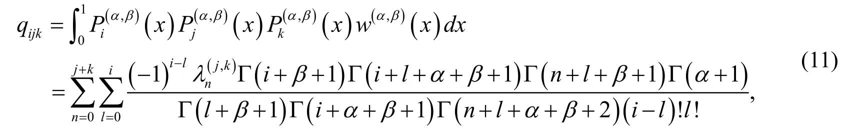
wherewere introduced in Lemma 1.

2.3 Function approximation

A three-variable continuous functionin the domaincan be expanded in terms of three-variable shifted Jacobi polynomials as

where

In practice, thetruncated series with respect to all three variablesx, y andz can be used an approximation for the given function

whereandare the unknown coefficients and three-variable Jacobi polynomials vectors are defined as

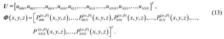
The following property of the product of two vectorsandis introduced and applied in solving the three-dimensional PDEs with variable coefficients.

whereandare, respectively,vector andoperational matrix of product.

Theorem 2. The entries of the matrixV , in Eq. (14), are computed as:

where qijkare introduced by Lemma 2.

Proof. See Sadri et al. [Sadri, Amini and Cheng (2017)].

3 The differential operational matrix of one-variable shifted Jacobi polynomials vector

Lemma 3. The first-order derivative of the vector （）

Φx can be expressed by

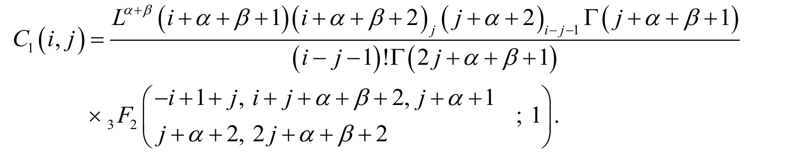
whereis theoperational matrix of derivative given by

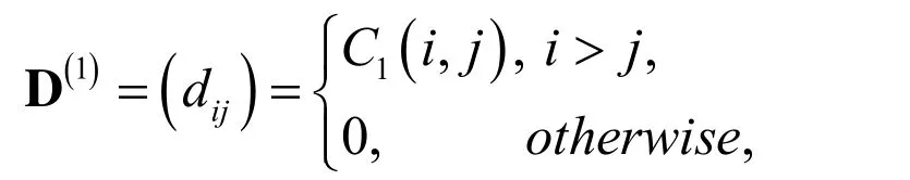
where

For the proof see Doha et al. [Doha, Bhrawy and Ezz-Eldien (2012)].

Theorem 3. Let （）x Φbe one-variable shifted Jacobi polynomials vector and let alsov＞0,then

whereis theoperational matrix of derivative of orderv in the Caputo sense and is defined by:

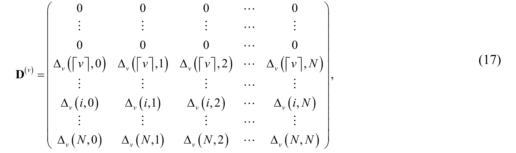
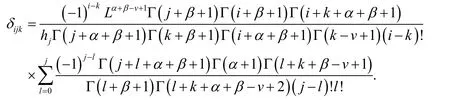
where

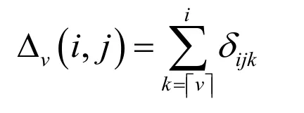
and δijkis given by

Note that inthe firstrows, are all zeros.

Proof. See Doha et al. [Doha, Bhrawy and Ezz-Eldien (2012)].

4 Error bound and convergence analysis

In this section, we show that the given method in the previous sections, is convergent. For our purpose we will need the following definitions and theorems to obtain an error bound for the proposed method in the Jacobi-weighted Sobolev Space.

Definition 4. We define

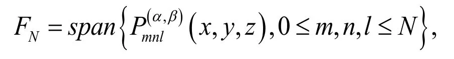
as the finite-dimensional polynomials space.

Theorem 4. Suppose thatis the Jacobi approximate solution tofromandis the Taylor series of theof order N respect to each variables x, y and z, then an error bound can be presented as follows:

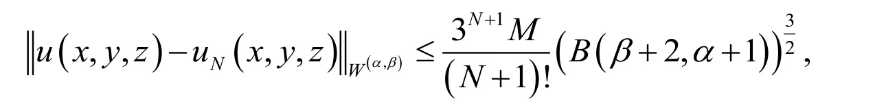
where

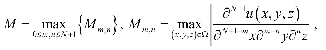
andis the well-known Beta function.

Proof. See Sadri et al. [Sadri, Amini and Cheng (2017)].

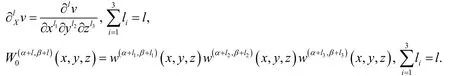
Definition 5. To derive approximation results, we introduce the Jacobi-weighted Space:

equipped with the following norm and semi-norm:

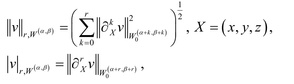
where

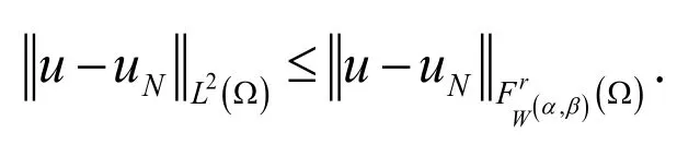
Theorem 5. For anyandthe following estimate holds:

whereis a positive constant independent of any function,N,αand.

Proof. See Sadri et al. [Sadri, Amini and Cheng (2017)].

Remark. Letand

∈be the Jacobi approximation to u . Then,the following estimates holds for all

5 Numerical implementation

In the section, we use the three-variable shifted Jacobi polynomials to solve threedimensional fractional-order PDEs with variable coefficients.

Similarity, the functionsandare also approximated by the three-variable shifted Jacobi polynomials as:

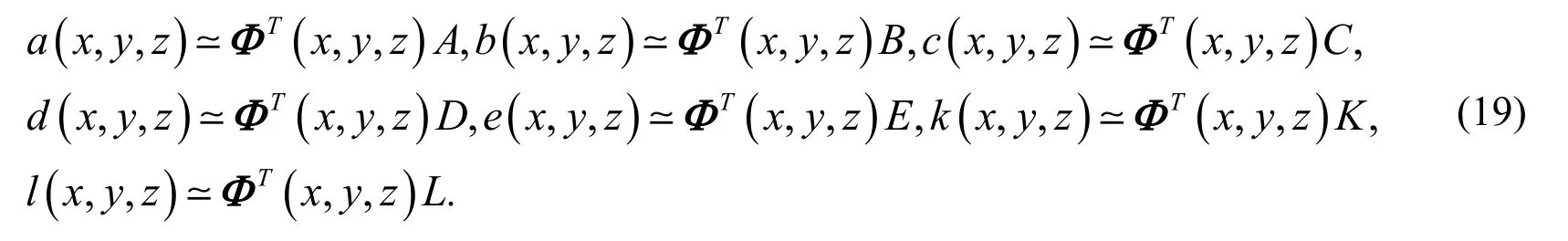
whereandcan be obtained by Eq. (13).

Using Eqs. (12), (14), (15) and (16) we have Sadri et al. [Sadri, Amini and Cheng (2017)]

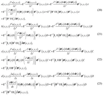
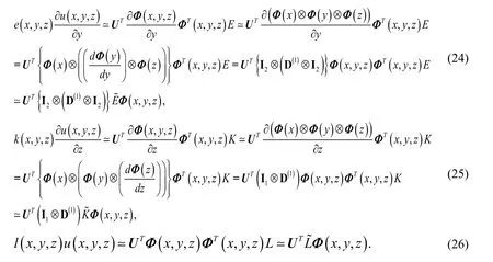
whereandareandidentity matrices,respectively. Substituting Eqs. (20)-(26) into Eq. (1) we get

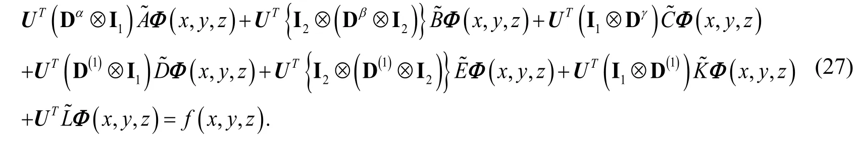
For the Dirichlet boundary condition (2) we have

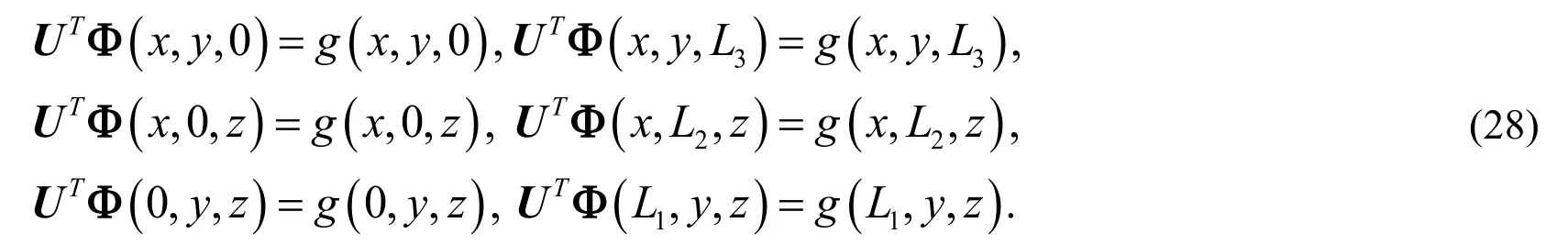
Eq. (27) together with Eq. (28) constitutes a system of algebraic equations. Then dispersing the unknown variables x, y and z as the following way:

Then we have

Solving this system, the unknown coefficient matrix U can be obtained. Then using Eq.(12), the unknown solution function （ ）,,u x y z is found.

6 Numerical experiments

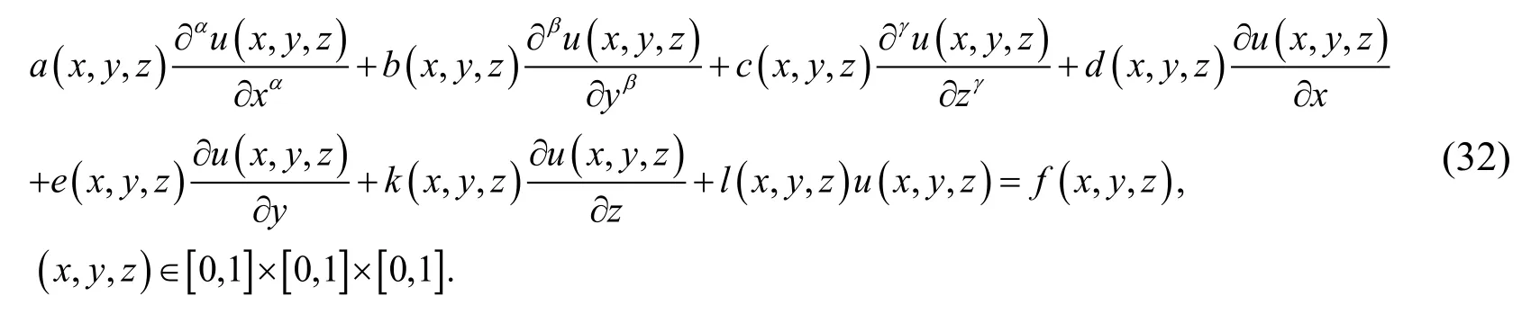
Example 1. Consider the following three-dimensional multi-term fractional-order PDEs with variable coefficients

with the Dirichlet boundary conditions:The analytical solution of this problem isWhenN=2,4and 6, the absolute errors at some values of x, y and z are shown in Tab. 1. Tab. 1 shows that the absolute errors decrease as N increases.

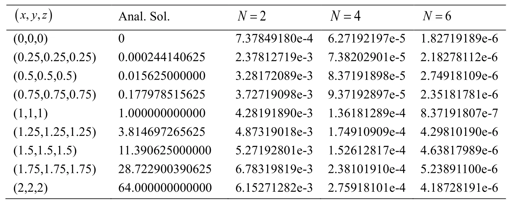
Table 1: The absolute errors at some values of x, y, z with 2,4,6 N=

Example 2. Consider the following three-dimensional fractional-order PDEs with variable coefficients

where

andSubject to the Dirichlet boundary conditions:The analytical solution of this problem isExample 2 and Example 3 show that the numerical solutions approximate to the exact solutions well asN becomes bigger.

(i) WhenWhenN=3,4and5, the graphs of the numerical solutions atand 0.9 are shown in Fig. 1.

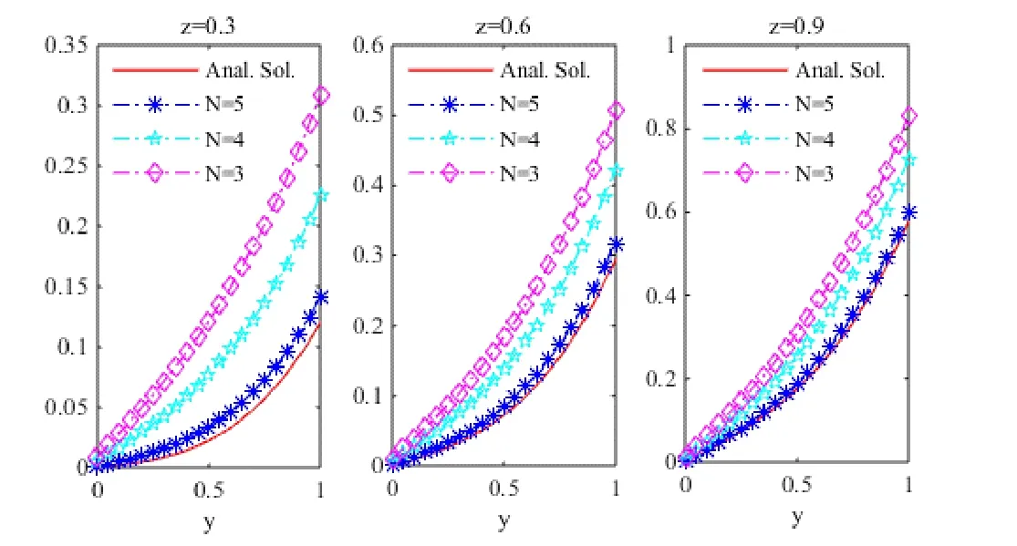
Figure 1: The numerical solution0.3,0.6=and 0.9 when N=3,4and 5

(ii) WhenWhen N=3,4and 5, the graphs of the numerical solutions atand 0.9 are shown in Fig. 2.

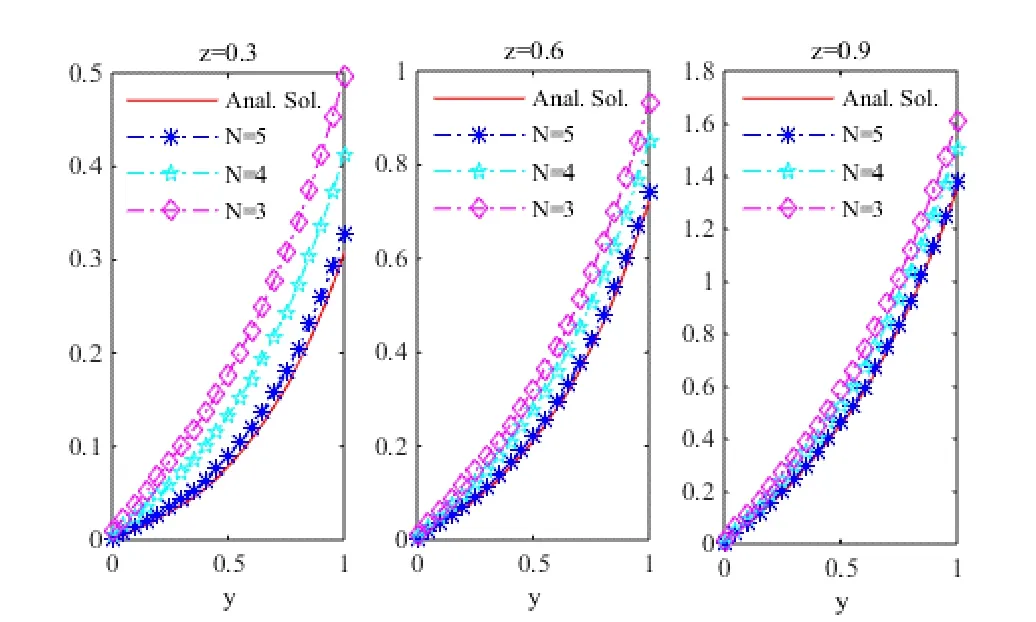
Figure 2: The numerical solutionat and 0.9 when N=3,4and 5

Example 3. Consider the following three-dimensional second-order PDEs with variable coefficients

whereandWith the Dirichlet boundary conditions:

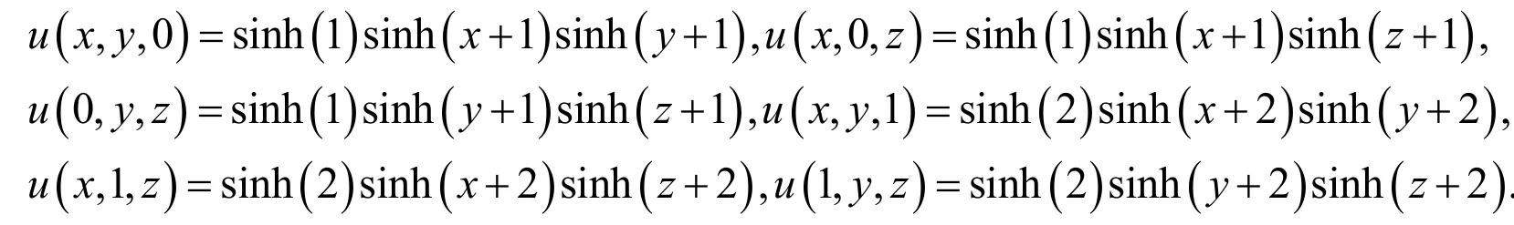
The analytical solution of this problem is

whenThe graphs of the numerical and analytical solutions whenN=2,3and 4 are shown in Figs. 3-6.

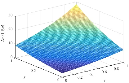
Figure 3: Analytical solution

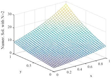
Figure 4: Numerical solution with N=2.

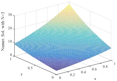
Figure 5: Numerical solution with N=3.

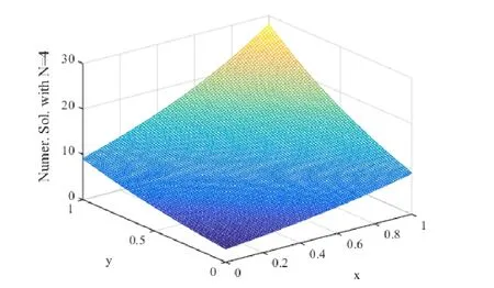
Figure 6: Numerical solution with N=4.

Example 4. Consider Eq. (33), we define the 2-norm error as

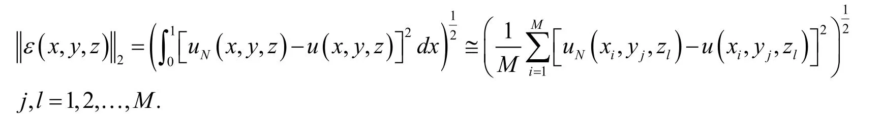
Whereandare the approximate and exact solutions respectively.

Whenandthe 2-norm error

with M=21 atare shown in Tab. 2. Tab. 2 shows that the numerical precision can achieveonly small series terms are expanded.

Table 2: The 2-norm errorwith N=2,3and 4

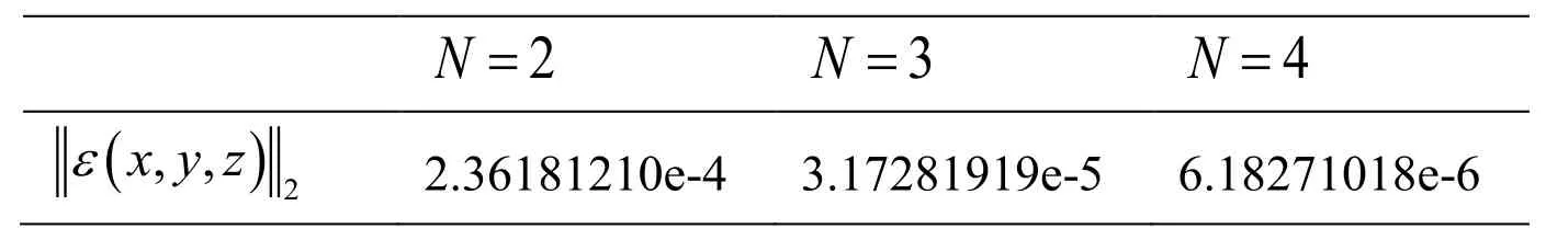
Table 2: The 2-norm errorwith N=2,3and 4

2 N=N=3N=4（ ）2 x, y, z ε 2.36181210e-4 3.17281919e-5 6.18271018e-6

7 Conclusions

In this article we have studied a numerical scheme to solve three-dimensional multi-term fractional-order PDEs with variable coefficients. Our approach is based on the threevariable shifted Jacobi polynomials and their operational matrices of fractional derivatives together with a set of suitable collocation nodes. The approximation of the solution together with imposing the collocation nodes is utilized to reduce the computation of this problem to some algebraic equations. The numerical results show that our method is convergent as N increases.

Acknowledgement:This work was supported by the Collaborative Innovation Center of Taiyuan Heavy Machinery Equipment, Postdoctoral Startup Fund of Taiyuan University of Science and Technology (20152034), the Natural Science Foundation of Shanxi Province(201701D221135), National College Students Innovation and Entrepreneurship Project(201710109003) and (201610109007).

Abushama, A.; Bialecki, B.(2008): Modified nodal cubic spline collocation for Poisson equation. Society for Industrial and Applied Mathematics, vol. 46, pp. 397-418.

Arpaci, V.(1984): Convection Heat Transfer. Prentice Hall, New Jersey.

Aziz, I.; Asif, M.(2017): Haar wavelet collocation method for three-dimensional elliptic partial differential equations. Computers & Mathematics with Applications, vol. 73, no. 9,pp. 2023-2034.

Bhrawy, A. H.; Zaky, M. A. (2015): A method based on the Jacobi tau approximation for solving multi-term time-space fractional partial differential equations. Journal of Computational Physics, vol. 281, pp. 876-895.

Boisvert, R.(1981): Families of high order accurate discretizations of some elliptic problems. Siam Journal on Scientific & Statistical Computing, vol. 2, pp. 268-284.

Borhanifar, A.; Sadri, K.(2015): A new operational approach for numerical solution of generalized functional integro-differential equations. Journal of Computational and Applied Mathematics, vol. 279, pp. 80-96.

Britt, S.; Tsynkov, S.; Turkel, E.(2010): A compact fourth order scheme for the Helmholtz equation in polar coordinates. Journal of Scientific Computing, vol. 45, pp. 26-47.

Cebeci, T.(2002): Convection Heat Transfer. Horizons Publishing Inc., Springer, Long Beach, California, Heidelberg.

Ciarlet, P.(2002): The finite element method for elliptic problems. North Holland.

Dehghan, M.; Shirzadi, M.(2015): Numerical solution of stochastic elliptic partial differential equations using the meshless method of radial basis functions. Engineering Analysis with Boundary Elements, vol. 50, pp. 291-303.

Doha, E. H.; Bhrawy, A. H.; Ezz-Eldien, S. S.(2012): A new Jacobi operational matrix:An application for solving fractional differential equations. Applied Mathematical Modelling, vol. 36, no. 10, pp. 4931-4943.

Fairweather, G.; Karageorghis, A.; Maack, J.(2011): Compact optimal quadratic spline collocation methods for the Helmholtz equation. Journal of Computational Physics, vol.230, pp. 2880-2895.

Ghimire, B. K.; Tian, H. Y.; Lamichhane, A. R.(2016): Numerical solutions of elliptic partial differential equations using Chebyshev polynomials. Computers & Mathematics with Applications, vol. 72, no. 4, pp. 1042-1054.

Hu, H.; Li, Z.; Cheng, D.(2005): Radial basis collocation methods for elliptic boundary value problems. Computers & Mathematics with Applications, vol. 50, pp. 289-320.

Mittal, R. C.; Dahiya, S.(2017): Numerical simulation of three-dimensional telegraphic equation using cubic B-spline differential quadrature method. Applied Mathematics &Computation, vol. 313, pp. 442-452.

Myint-U, T.; Debnath, L.(2007): Linear partial differential equations for scientists and engineers. Birkhauser.

Roache, P.(1972): Computational fluid dynamics. Hermosa Press, Albuquerque, New Mexico.

Sadri, K.; Amini, A.; Cheng, C.(2017): Low cost numerical solution for threedimensional linear and nonlinear integral equations via three-dimensional Jacobi polynomials. Journal of Computational & Applied Mathematics, vol. 319, pp. 493-513.

Shiralashetti, S. C.; Kantli, M. H.; Deshi, A. B.(2016): New wavelet based fullapproximation scheme for the numerical solution of nonlinear elliptic partial differential equations. Alexandria Engineering Journal, vol. 55, no. 3, pp. 2797-2804.

Singer, I.; Turkel, E.(2006): Sixth order accurate finite difference schemes for the Helmholtz equation. Journal of Computational Acoustics, vol. 14, pp. 339-351.

Spotz, W.; Carey, G.(1996): A high-order compact formulation for the 3D Poisson equation. Numer. Methods Partial Differential Equations, vol. 183, pp. 235-243.

Srivastava, V. K.; Awasthi, M. K.; Chaurasia, R. K.(2017): Reduced differential transform method to solve two and three dimensional second order hyperbolic telegraph equations.Journal of King Saud University Engineering Sciences, vol. 29, no. 2, pp. 166-171.

Wang, J.; Zhong, W.; Zhang, J.(2006): A general meshsize fourth order compact difference discretization scheme for 3D Poisson equation. Applied Mathematics &Computation, vol. 183, pp. 804-812.

Zhang, K.; Zhang, R.; Yin, Y.(2008): Domain decomposition methods for linear and semilinear elliptic stochastic partial differential equations. Applied Mathematics &Computation, vol. 195, no. 2, pp. 630-640.

Zhao, F.; Huang, Q.; Xie, J.; Li, Y.; Ma, M. et al.(2017): Chebyshev polynomials approach for numerically solving system of two-dimensional fractional PDEs and convergence analysis. Applied Mathematics & Computation, vol. 313, pp. 321-330.