NIE Yongfangand ZHANG Tao

1.Department of Automation,Tsinghua University,Beijing 100084,China;2.Department of Strategic Missile and Underwater Weapon,Naval Submarine Academy,Qingdao 266071,China

1.Introduction

Mahler settled the traditional data association difficulty in the multiple-target tracking field by proposing random finite set(RFS)theory[1].The individual targets and observations are viewed as two RFSs in a Bayesian filtering framework[2].As a recursive solution to solve the abovementioned RFS-estimation problem,the probability hypothesis density(PHD) filter[3]can solve the data association difficulty in a single-targetstate space,which is more appropriate for strong clutter scenarios.However,there is no closed-form solution for the PHD filter in view of its multiple integrals.Therefore,the sequential Monte Carlo PHD(SMC-PHD) filter[4–6]was proposedbyVo et al.to obtain the tractable closed-form solutions.The SMC-PHD filter needs a large number of particles,and it is unreliable when extracting state estimates using clustering techniques.Thereafter,the Gaussian mixture PHD(GM-PHD)filter[7]was proposed by Vo et al.for the linear Gaussian model.Meanwhile,they extended this solution to nonlinear target models combined with the extended Kalman filter(EKF)and the unscented Kalman filter(UKF).This filter has been widely applied in multi-target tracking,e.g.,as Doppler,sonar images and pedestriandetection[8–11].

Compared with the SMC-PHD filter,the GM-PHD filter can extract state estimates from the posterior intensity efficiently and reliably.However,with the increment of the number of Gaussian components,so does the computation cost of the GM-PHD filter.Therefore,the low weighted Gaussian components are pruned and the close ones are merged into a single Gaussian component in the GM-PHD filter.Despite reducing the computational load,this method is not appropriate to deal with close proximity targets.Therefore,it is important to enhance the estimate accuracy of the GM-PHD filter for some proximity targets.Chen et al.proposed an algorithm[12]to solve this problem by two merging steps according to whether the rounded value of the sum of the first merged weights is greater than one.However,in some cases,this approach cannot break while-loop at the second merging step.This paper,therefore,based on their theory,proposes an improved algorithm.The improved algorithm does not need two merging steps,which solves the end-less while-loop problem and saves the running time.Simulation results demonstrate that this improved algorithm is more robust and easier to implement than the formal one.

2.Problem statements

2.1 GM-PHD filter

This paper only refers to linear Gaussian multiple-target models and assumes there is no target spawning for the GM-PHD filter[7].

Consider a linear system model as follows:

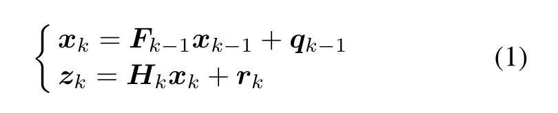
whereFk-1andHkare the state transition and measurement matrix,respectively.qk-1is the process noise with covarianceQk-1.rkis the measurement noise with covarianceRk.

Each target is a linear Gaussian model as follows:

where fk|k-1and θkare the transition density and the likelihood function,respectively.N denotes a Gaussian density.

There are three steps in the GM-PHD filter:prediction and updating,pruning,and state extraction.The following section gives the prediction and updating step.

Assume at time k-1 the posterior intensityvk-1is the Jk-1Gaussian components mixture as follows:

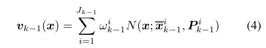
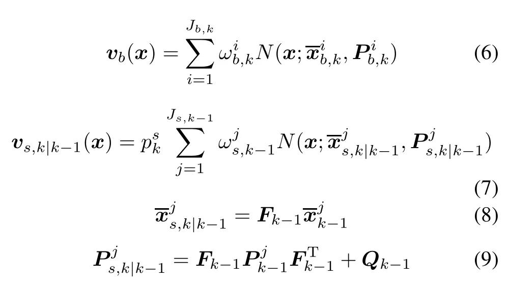
Then,we can give the predicted intensity at time k.

wherevb,k(x)andvs,k|k-1(x)are the birth intensity and surviving intensity as follows:

Therefore,at time k,the predicted and posterior intensities are both Gaussian mixture forms as follows:

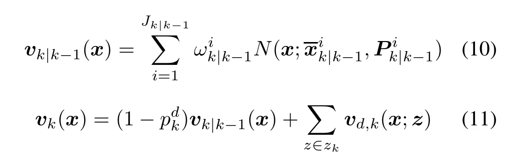
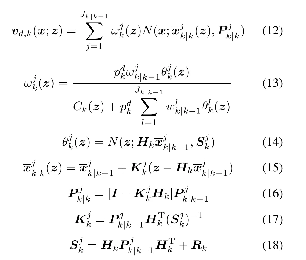
In(13),Ck(z)is the clutter intensity,which is usually assumed as a Poisson distributed RFS.

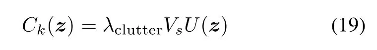
where λclutteris the clutter rate,Vsrefers to the volume of the measurement region,and U(·)is a uniform density.

2.2 GM-PHD filter pruning procedure

As time k increases,so does the computation cost of the GM-PHD filter because of the increasing number of Gaussian components.To representvk,the GM-PHD filter uses JkGaussian components at time k,where

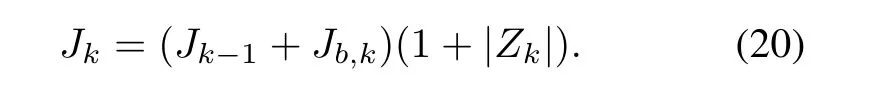
From(20),we know that Jkwill increase without bound.

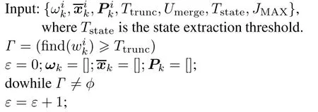
The GM-PHD filter uses a pruning procedure to reduce Jk.This can be done by discarding those Gaussian components whose weights are below some preset truncation threshold Ttruncand merging those Gaussian components whose distances between each other are below the preset Mahalanobis distance threshold Umergeintoone.The pruning algorithm is described as follows[7],where JMAXdenotes the maximum allowable number.

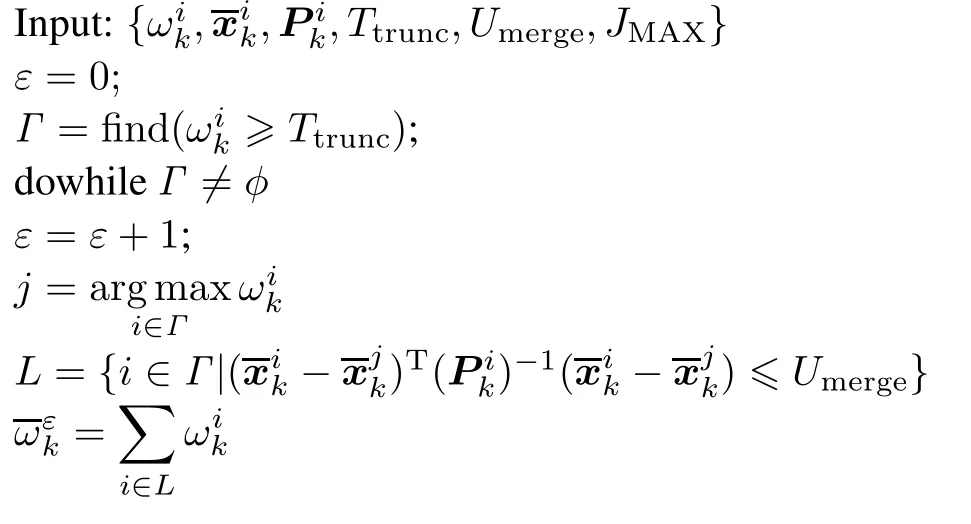
end while

Jk=ε

3.Improved pruning algorithm for the GM-PHD filter

In the pruning algorithm of the GM-PHD filter,the merging criterion only utilizes means and covariances of each Gaussian component,

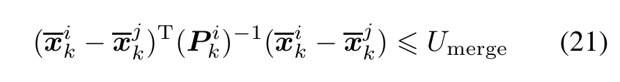
whereas the weight of each component is not considered.Therefore,this pruning algorithm cannot distinguish the close proximity targets whose distances are smaller than the merging threshold but their weights are big.In fact,they actually represent different targets.In such cases,the estimate precision of the GM-PHD filter will deteriorate.This problem is particularly serious in the strong clutter environment.

3.1 Problem of the pruning algorithm in[12]

In[12],the authors proposed a merging algorithm to solve the previous problem.They merge the components depending on a new condition which utilizes all three parameters of the components and two merging steps according to whether the rounded value of the sum of the first merged weights Q is greater than 1.If this condition is not satisfied,which represents only one target,just do the first merging step according to the procedure of the pruning algorithm.Otherwise there will be more than one target with the same weights.It is necessary to run the second merging step according to the following merging criterion.

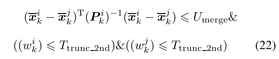
The detail procedure can be seen in[12].For easily understanding the whole paper,we only describe the second merging algorithm as follows:

Do the same procedure of the pruning algorithm if Q＞1

Replace the merging criterion L with L2nd

end while

Unfortunatly,this second merging step is an end-less while-loop in some cases because the merging criterion is stricter than the first one.

Let us consider a very simple example:

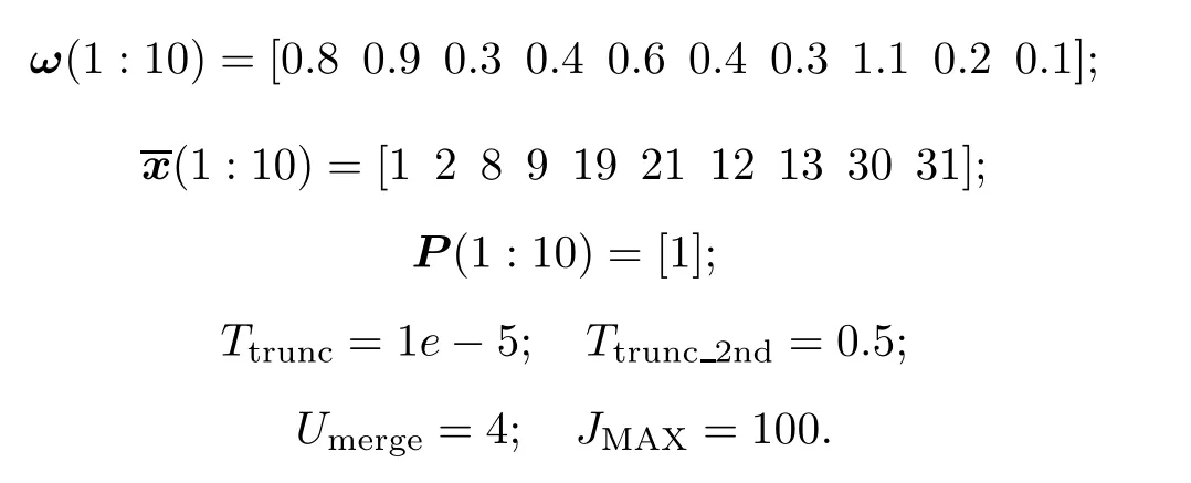
Obviously,onlyω=[0.3,0.4,0.2,0.1]satisfies the second merging criterion in[12].Therefore,Γ /= φ is always satisfied and the while-loop will never stop.

3.2 Improved pruning algorithm

Based on the ground of[12],an improved pruning algorithm is proposed to solve the above problems.The detail procedure is as follows.

Step 1Input the posterior intensity result of the GMPHD filter and the corresponding threshold parametersat time k.

Step 2Truncate those Gaussian components whose weights are lower than the threshold Ttrunc.The result is denoted as Γ = fi nd(≥ Ttrunc).

Step 3Using(21),divide Γ into ε groups,each has L Gaussian components.

Step 4Calculate the valuesQ(ε)=round(sum()).If Q(ε) ＞ 1 and＞ Tstate,do not merge the L Gaussian components into one,and keep them as the different targets,otherwise do the same procedure of the pruning algorithm,sum the weights=sum()and merge the corresponding,

Step 5Append the result of each ε into the initial matrix.

Step 6When the number of the Gaussian components is larger than JMAX,replace the previous result with the JMAXlargest weight Gaussian components.

Step 7Output the final Gaussian components as the pruned posterior intensityvkpropagated to the time step k+1.

We describe the corresponding pseudo-code as follows.

endwhile

Jk=size(ωk,2)

Consider the previous simple example,we can get five Gaussian components pruning according to the algorithm.However,if we utilize the improved pruning algorithm,we can get six Gaussian components.The first and second components are selected as two different targets rather than merged into one.Thus,we can avoid the end-less problem and save the running time obviously without the need of the second merging step in[12].

4.Example and simulation results

4.1 Example

4.1.1 Simulation parameters

Consider a four-dimensional simulation scenario.The length and width of the simulation region with clutter are both 1 000 m.The quantity of the measurement targets is unknown and time-varying.At time k,the state vector isand the measurement vector isThe sample period is T=1 s.The other system simulation parameters are as follows:

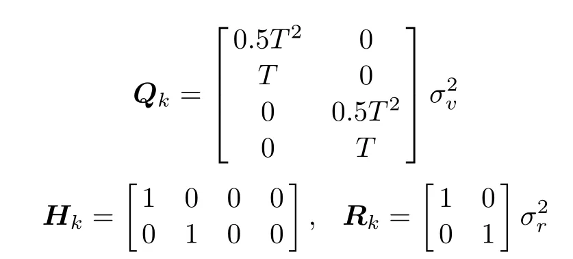
where σq=3 m/s2and σr=5 m are the corresponding noise standard deviations,respectively.

The birth intensityvb,k(x)is set as the following Poisson RFS:

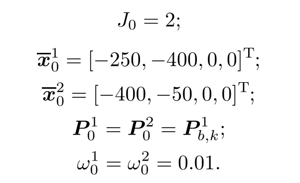
where=[15,-250,0,0]Tis the first birth target mean and=[-5,-240,0,0]Tis the second one.

The corresponding birth covariance is as follows:

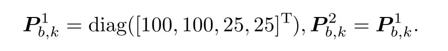
The initial Gaussian components are given as follows:

The clutter parameters are λclutter=20 × 10-6m-2and Vs=106m2.

The pruning parameters are Ttrunc=1e-5,Umerge=4,Tstate=0.5 and JMAX=100.

The detection and survival probability parameters are=0.98 and=0.99.

Target1and target2st art at k=1s whiles to patk=50s and k=35 s,respectively.Target 3 and target 4 start at k=25 s and stop at k=50 s,which denote the close proximity targets in this simulation example.

4.1.2 Performance evaluation parameters

Optimal sub-pattern assignment(OSPA)is a consistent metric for performance evaluation of multi-object filters[13,14].

The distance between two arbitrary RFSs X1,X2∈W is given by Dcu(X1,X2):=min(cu,D(X1,X2))as follows:

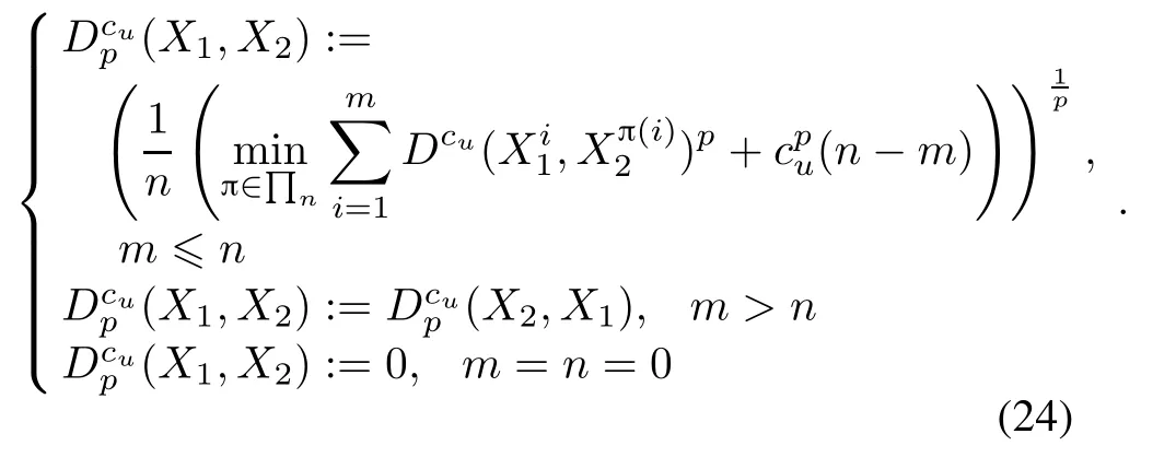
There are two free parameters in OSPA metric which can be adjusted by the user.Order p∈[1,∞)is the out lier sensitivity,and cut-off cu＞0 is the cardinality penalty.The detail meanings of other parameters in(24)can be seen in[13].In this paper,p=2 is selected because it can yield the smooth distance curve.The cut-off parameter is set as cu=100.

4.2 Simulation results

As can be easily seen from Fig.1,the GM-PHD filter cannot distinguish the close proximity target 3 and target 4,which are merged into one at almost every step.Moreover,this results in the target number estimation errors in Fig.2 and the bigger OSPA metric errors in Fig.3.

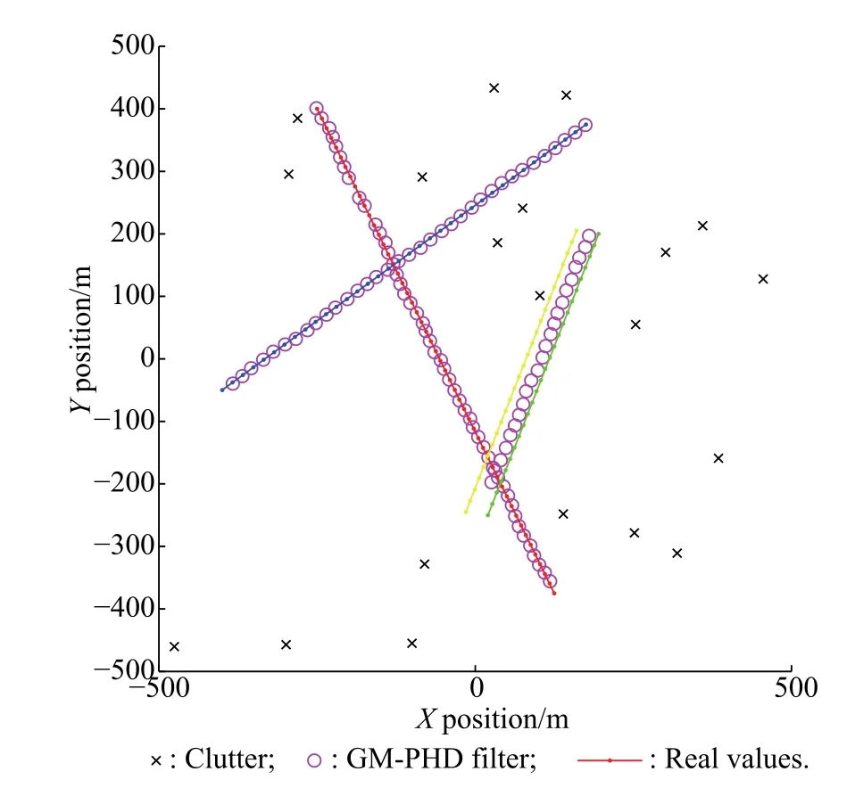
Fig.1 GM-PHD filter simulation results

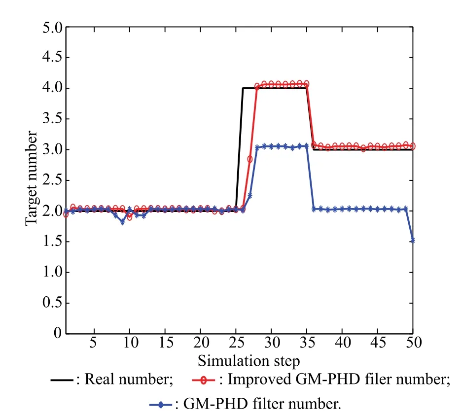
Fig.2 Target number estimation results

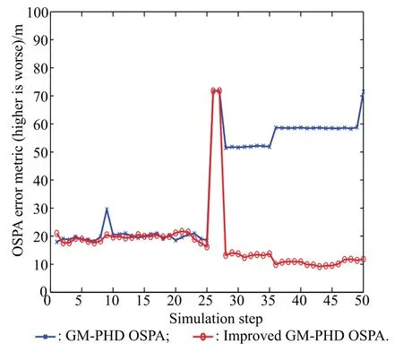
Fig.3 OSPA error metric estimation results

As can be seen from Fig.4,the improved GM-PHD filter can get more precise state estimation.Although there are still big target number errors at time k=25 s,26 s,which are caused by the new born targets that cannot be detected immediately.The following steps give better state estimation than the GM-PHD filter does.Simulation results of Fig.2 and Fig.3 also demonstrate that the estimation precision of the improved GM-PHD filter outperforms that of the GM-PHD filter in the close proximity targets environment.

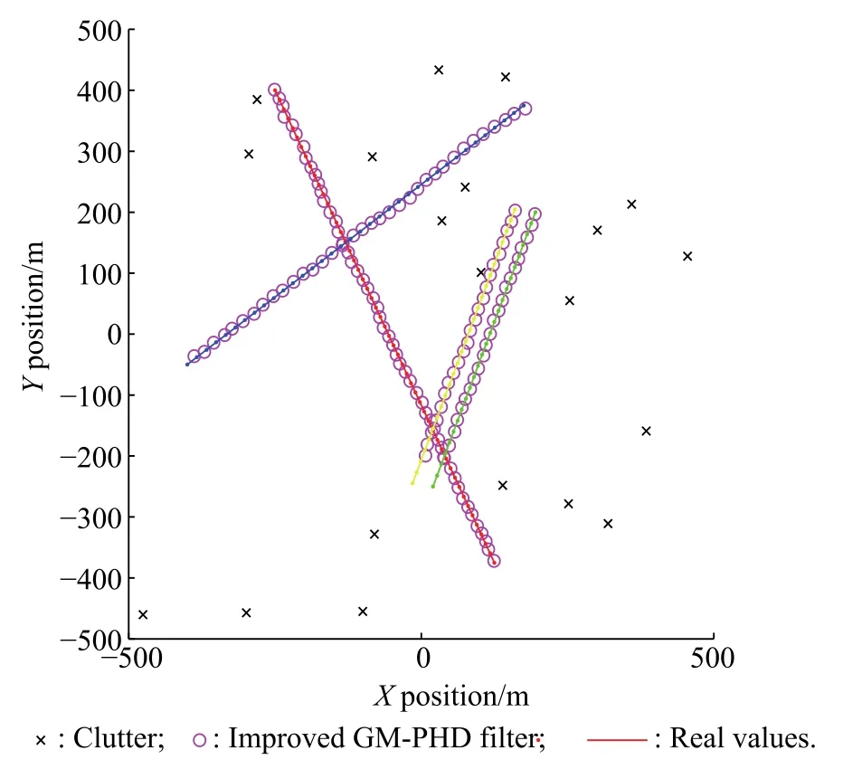
Fig.4 Improved GM-PHD filter simulation results

As we all know,the main reason that results in the measurement uncertainty is the clutter.Therefore,the clutter density[15]is an important evaluation criterion for a clutter environment.It is defined as the average clutter number in the measurement region which is uniformly distributed.To compare the robustness of the two kinds of GM-PHD filters,we simulate the average OSPA error metric for different clutter rates.The corresponding simulation results ranging from λclutter=0 to λclutter=10-4m-2are plotted in Fig.5.

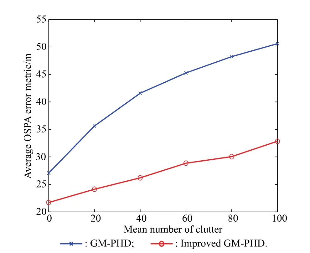
Fig.5 OSPA average errors metric for various mean numbers of clutter

It can be seen from Fig.5 that as the clutter rates increase,so do the average OSPA error metrics of the GMPHD filter and the improved GM-PHD filter.However,the latter gives a smaller average OSPA error metric than the former at each clutter rate.This result demonstrates that the improved GM-PHD filter is more robust in a complex clutter environment.The main reason is the improved GM-PHD filter can track the target state with a more effective pruning procedure for the close proximity targets.

5.Conclusions

To solve the increasing Gaussian components problem of the GM-PHD filter in the strong clutter environment,an improved pruning algorithm is proposed in this paper to increase the estimate accuracy of the GM-PHD filter when it is used in close proximity targets tracking.This algorithm avoids the actually different targets whose distances are below the merging threshold being merged into one.Its pruning criterion utilizes not only the Gaussian components’means and covariance,but their weights.More importantly,although based on the same ground,this algorithm solves the end-less while problem and does not need two merging steps which are needed in the similar literature.It can save the running time obviously.Simulation results show that this improved pruning algorithm is more robust and easier to implement than the formal one.The following research will focus on solving how to detect the new born targets immediately and the GM-PHD filter in the unknown clutter environment.

Acknowledgment

The authors would like to thank Bryan Clarke for providing the GM-PHD filter Matlab source code.

[1]MAHLER R.Multi-target filtering via first-order multi-target moments.IEEE Trans.on Aerospace and Electronic Systems,2003,39(4):1152–1178.

[2]MAHLER R.Advances in statistical multisource-multitarget information fusion.Boston:Artech House,2014.

[3]MAHLER R.PHD filters of higher order in target number.IEEE Trans.on Aerospace and Electronic Systems,2007,43(4):1523–1543.

[4]VO B N,SINGH S,DOUCET A.Sequential Monte Carlo implementation of the PHD filter for multi-target tracking.Proc.of the 6th Conference on Information Fusion,2003:792–799.

[5]VO B N,SINGH S,DOUCET A.Sequential Monte Carlo methods for multi-target filtering withrandom finitesets.IEEE Trans.on Aerospace and Electronic Systems,2005,41(4):1224–1245.

[6]RISTIC B.Particle filters for random set models.New York:Springer,2013.

[7]VO B N,MA W.The Gaussian mixture probability hypothesis density filter.IEEE Trans.on Signal Processing,2006,54(11):4091–4104.

[8]WU W H,LIU W,JIANG J,et al.GM-PHD filter-based multitarget tracking in the presence of Doppler blind zone.Digital Signal Processing,2016,52(C):1–12.

[9]CLARK D.GM-PHD filter multitarget tracking in sonar images.Proc.of Defense and Security Symposium:International Society for Optics and Photonics,2006,6235:62350R-62350R-8.

[10]EDMANV,ANDERSSON M,GRANSTROM K,et al.Pedestrian group tracking using the GM-PHD filter.Proc.of IEEE Signal Processing Conference,2013:1–5.

[11]ULMKE M,ERDINC O,WILLETT P.GMTI tracking via the Gaussian mixture cardinalized probability hypothesis density filter.IEEE Trans.on Aerospace and Electronic Systems,2010,46(4):1821–1833.

[12]CHE L,CHEN Z,YIN F.A novel merging algorithm in Gaussian mixture probability hypothesis density filter for close proximity targets tracking.Journal of Information&Computational Science,2011,8(12):2283–2299.

[13]SCHUHMACHER D,VO B T,VO B N.A consistent metric for performance evaluation of multi-object filters.IEEE Trans.on Signal Processing,2008,56(8):3447–3457.

[14]RISTIC B,VO B N,CLARK D.A metric for performance evaluation of multi-target tracking algorithms.IEEE Trans.on Signal Processing,2011,59(7):3452–3457.

[15]MULLANE J,VO B N,ADAMS M,et al.Random finite sets for robot mapping and SLAM.Berlin:Springer,2011.