Feng-Guang Li(李風光),Wan-Su Bao(鮑皖蘇),,? Xiang Wang(汪翔),Xiang-Qun Fu(付向群), Shuo Zhang(張碩),Yu-Tao Du(杜宇韜),Tan Li(李坦),and Bo-Wen Ma(馬博文)1Zhengzhou Information Science and Technology Institute,Zhengzhou 450004,China

2Synergetic Innovation Center of Quantum Information and Quantum Physics,University of Science and Technology of China,Hefei 230026,China

1 Introduction

As a new alternative type of quantum computation,adiabatic quantum algorithm was proposed by Farhiet al.[1]It builds a problem Hamiltonian whose ground state encodes the solution of a problem,and an initial Hamiltonian whose ground state is known.Then it constructs a time-dependent Hamiltonian that evolves progressively from the initial Hamiltonian to the problem Hamiltonian.If the system begins with the ground state of the initial Hamiltonian and evolves slowly enough,the quantum adiabatic theorem[2]ensures that the system will evolve into the ground state of the problem Hamiltonian.Generally,the quantum adiabatic model is computationally equivalent to the quantum circuit model.[3]Because it has capacity to remain robust against environment noise,[4]the adiabatic quantum algorithm attracts more and more attention.[5?8]

In adiabatic quantum algorithm,the success rate can be defined as the fidelity between the actual time-evolved state(the solution of the Schr?dinger equation)and the instantaneous ground state,calculated at the final timeT.The adiabatic theorem states that if the evolution is perfectly adiabatic(i.e.the run timeT?1/ΔE2,where ΔEis the minimum gap between the lowest two eigenvalues),the success rate approaches one.But for a short run timeT＜1/ΔE2(hereafter,we denote it non-adiabatic evolution),the relation between the run time and success rate for non-adiabatic evolution algorithm is poorly understood.Most attention has been paid to calculate the ΔE,which close to the complexity of the quantum adiabatic algorithm.[9?10]Only little attention has been paid to the deviation from the adiabatic evolution.[11?14]In this paper,we study the success rate of local adiabatic quantum search algorithm[15]with an arbitrary finite run time.It means that the adiabatic condition is removed.What we cared is how the success rate change with arbitrary run time.

We study quantum dynamics of adiabatic search algorithm with an equivalent two-level system.We try to solve the time-independent Schr?dinger equation in quantum dynamics and obtain differential equations to calculate the success rate.The differential equations show that the success rate is closely related with the adiabatic parameters(t).Utilize the differential equations,we calculate numerically the success rate as a function of the run time in local adiabatic search algorithm.

Our paper is organized as follows:we brie fly introduce the quantum adiabatic search algorithm in Sec.2.The time-independent Schrodinger equation under nonadiabatic quantum dynamics is solved in Sec.3.In Sec.4,we give the function of success rate versus run time in local adiabatic search numerically.Finally,a conclusion is given in Sec.5.

2 Adiabatic Search Algorithm

Grover’s algorithm[16]solves an unstructured search problem in a time ofwhereNis the size of the database.And it is widely used in cryptography.[17]Its adiabatic version was also proposed.[10]In the search problem,the task is to locate the marked item out ofNunsorted items.We use a set of orthonormal basis|1〉,|2〉,...,|N〉to denote theNunsorted items and use|w〉to denote the marked item.According to the principle of adiabatic quantum computation,the corresponding problem Hamiltonian can be constructed as

Thus the target state|w〉is the ground state ofHp.The initial state can be prepared in an equal superposition of all could-be solutions:

thus the initial state is the ground state of the following initial Hamiltonian:

The change from the initial HamiltonianH0to the problem HamiltonianHpcan be done as

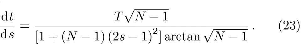
Heres(t)is a monotonic function withs(0)=0 ands(T)=1,whereTis the total run time.Generally,we choose a linear functions(t)=t/T,which called global path.In 2002,Roland proposed a local adiabatic search algorithm.[15]It does not use a linear function,but adapt the evolution rate ds/dtto the local adiabatic condition.The correspondings(t)satisfies

whereε? 1.Takes=1,

Hereafter,we denote it local path for convenience.Obviously,it satisfies the boundary conditions:whent=0,s=0,andH(s)=H0;Whent=T,s=1,andH(s)=H1.

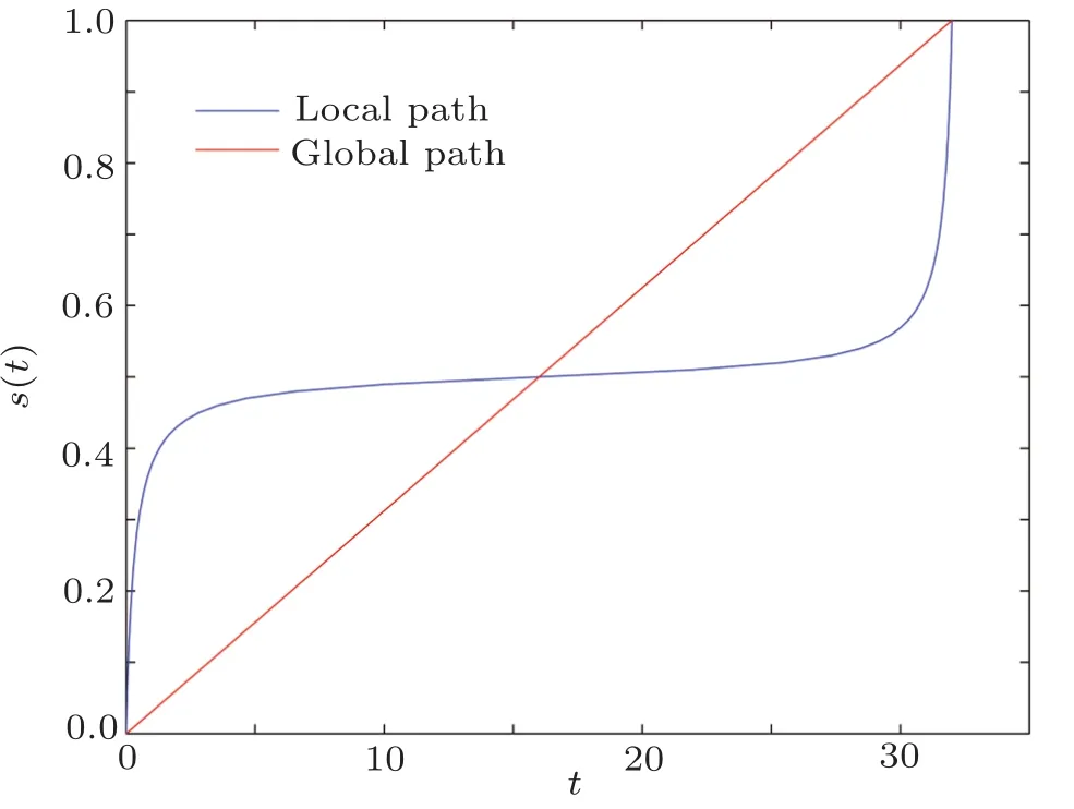
Fig.1 (Color online)The dynamic evolution path s(t)as a function of t for N=1024.The blue line corresponding to the local path and the red line corresponding to the global path s(t)=t/T.

For global path,paper[11,13]has studied the success rate versus run time.But for the local path,there is no research.In this paper,we propose a computation model for success rate and then apply it to local adiabatic search algorithm.

3 Success Rate in Adiabatic Search Algorithm

The first step is to obtain the expression of the instantaneous eigenstates of the time-dependent HamiltonianH(s(t)).[13]We representHs(t)with the orthonormal basis{|w〉,|w⊥〉}as

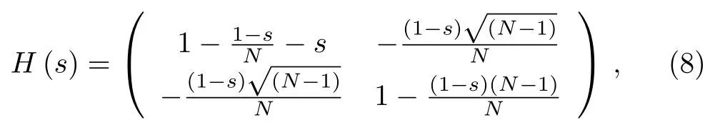
where Hamiltonian in Eq.(8)is written in convenient form as

whereZ(s) ≡ 2(1?s)+N(2s?1)andSince the first item is not relevant to dynamics,it will be dropped.The Hamiltonian can be written as

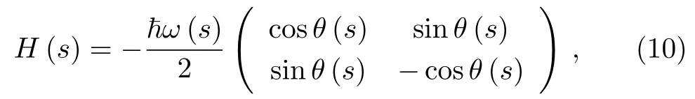
where the mixing angleθis defined by tanθ(s) ≡

X(s)/Z(s)andIt is easy to write down the instantaneous eigenstates ofH(s)|e±(s)〉=e±(s)|e±(s)〉,

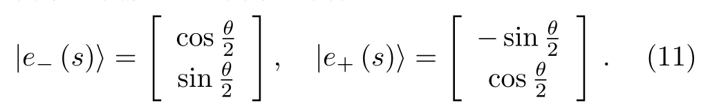
And the instantaneous eigenvalues are±(?ω(s))/2.Whens=1,thenθ=0 and|e?(1)〉=|w〉,corresponding to the marked item.

We can write the evolved state|φ(s(t))〉in terms of instantaneous eigenstates as

TheP(s)=a(s)2is the probability of system stay on the ground state|e?(s)〉,so the probabilityP(1)=|〈w||φ(1)〉|2=|〈e?(1)||φ(1)〉|2=a(1)2corresponding to the success rate.For arbitrary run time,we try to calculatea(s)by solving the time-dependent Schr?dinger equation

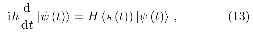
and obtain Theorem 1.

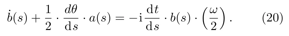
Theorem 1The probability amplitudea(s)andb(s)satisfy the follow differential equations:

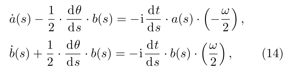
where˙a(s)and˙b(s)are first-order derivatives ofa(s)andb(s)respectively,and

Here dt/dsis determined by the paths(t).

ProofFrom i?(d/dt)|ψ(t)〉=H(s(t))|ψ(t)〉,we obtain

We calculate

and we have

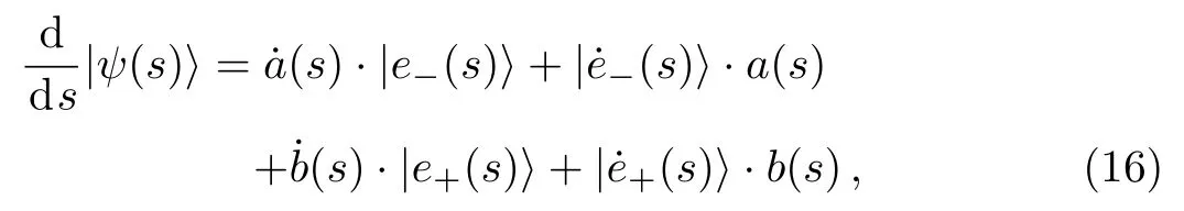
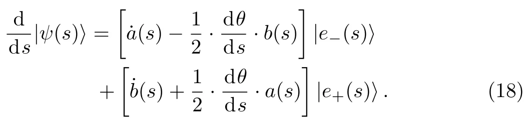
Substitute Eq.(17)into Eq.(16),we get

On the other hand,we know

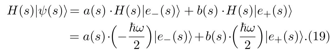
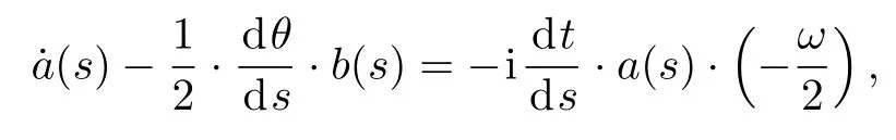
Substitute Eq.(19)and Eq.(18)into Eq.(15),we get

Here,θ=arctanX(s)/Z(s),then

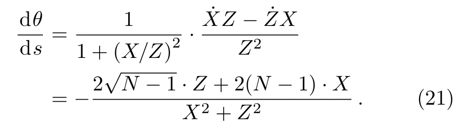
The theorem is hence proved.

If the path parameters(t)is given,then the dθ/ds,dt/dsandωcan be known.For arbitrary run timeT,we can calculate the success ratea(1)2numerically according to Theorem 1.

4 Success Rate Versus Run Time in Local Adiabatic Search Algorithm

From Theorem 1,we know dθ/ds,dt/dsandωare decided by the evolution functions(t).It means that for adiabatic search algorithm,if the size of databaseNand the run timeTis given,the success rate is completely depended ons(t).For local path and global path,we numerically calculate the success rateP(1)=a(1)2easily,and the result is shown in Fig.2.

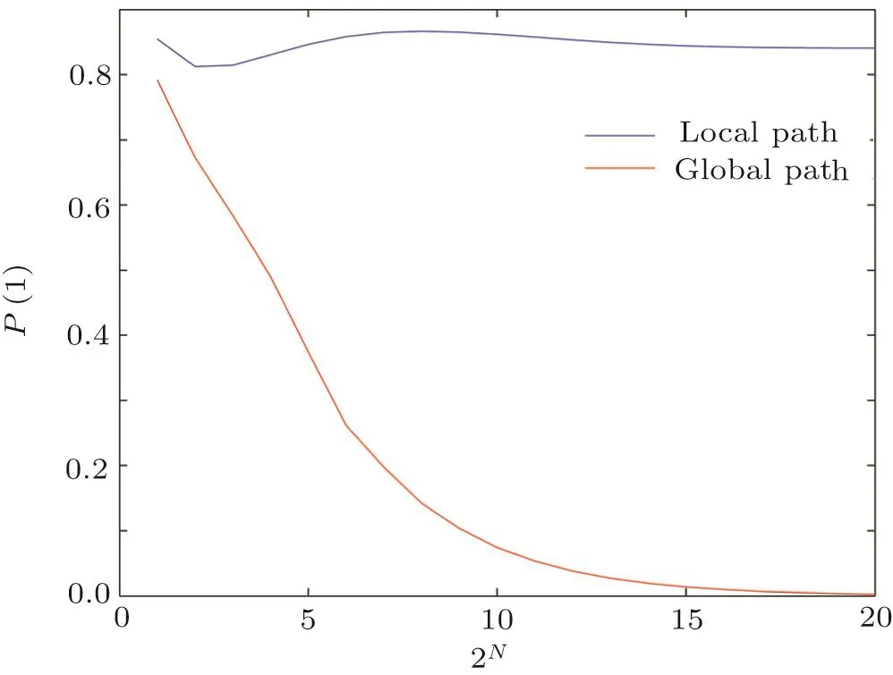
Fig.2 (Color online)The success rate P(1)as a function of the size of database N(from 1 to 220)for different path.Here is taken.

As depicted in Fig.2,for a given run timethe success rate decreases to 0 as the growing ofNin global adiabatic search algorithm but does not in local adiabatic.Because in global adiabatic search algorithm,Namely,whenthe evolution is non-adiabatic in global adiabatic search algorithm.So how the success rate changes with run timeTin local adiabatic search algorithm?

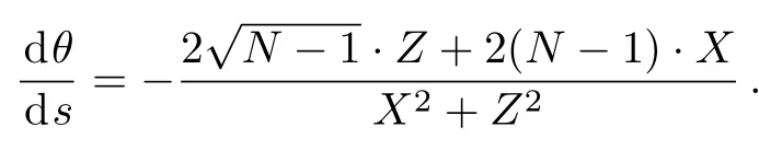
Here we study the success rate versus arbitrary run timeTin local adiabatic search algorithm utilizing Theorem 1.When

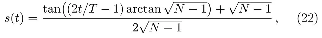
then

Substitute Eq.(23)into Eq.(14),we can numerically calculate the probability amplitudeP(s)=a(s)2easily.The result is shown in Fig.3.

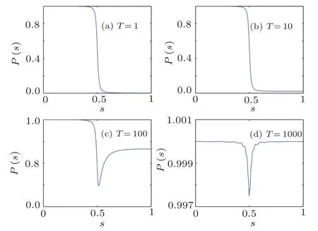
Fig.3 (Color online)The probability P(s)=a(s)2of being in the ground state as a function of s for different T=1,10,100,1000.Here the size of database N=1000 is taken.

For short run timeT,as shown in Figs.3(a)–3(b),the success rateP(1)is very small.But in Figs.3(c)–3(d),it approaches approximately to 1 for long run time.On the other hand,the error rate 1?P(1)=1?a(1)2=b(1)2is the transition probability ats=1.Rezakhaniet al.[11]found that the asymptotic form of 1?P(1)for the adiabatic quantum search from exponentially decay to the inverse-square decay.And the error rate versus run times in global adiabatic search was discussed by Ohet al.[13]Here,we give the error rate versus run times in local adiabatic search in Fig.4.

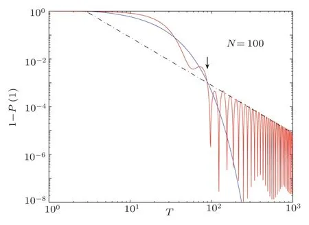
Fig.4 (Color online)Log-log plots of the error probability 1?P(1)as a function of T for N=100.The blue line is exp(?0.079T)and the black dashed line is 8/T2.The arrow indicates the critical run time Tc.

As shown in Fig.4,in local adiabatic search algorithm,the error probability 1?P(1)decreases exponentially for short run time and then decreases as inverse-square ofT.For different sizeN,we calculate numerically the error rate 1?P(1)as a function of the run timeTand find

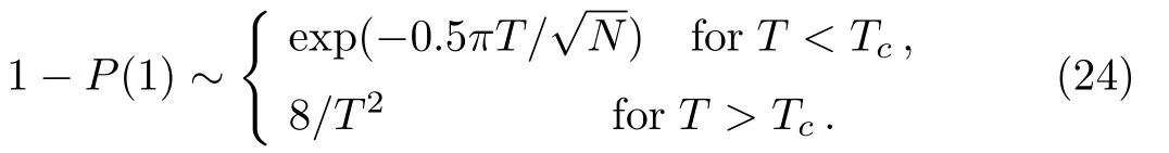
The critical run timeTcis a solution of the transcendental equation expSo the success rate

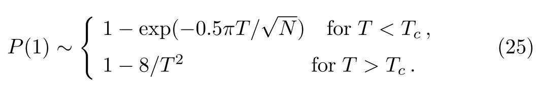
From the formula(25),we know the success rate is approximately equal to 1 for long run time and decreases exponentially for short run time.Furthermore,we calculate the success in different order of run timeT,the success rate as a function ofNas follows:

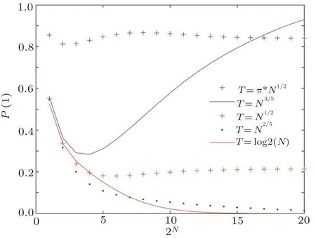
Fig.5 (Color online)The success rate P(1)as a function of the size of database N for different order of run time T.Here,the value of N is range from 1 to 220.

We explain the phenomenon in Fig.5 utilizing the formula(25).For arbitrary order of run timeT=Nk,k＞0,we have

Whenk＜0.5,then

It indirectly verifies the conclusion thatis optimal in local adiabatic search algorithm.[15]

5 Conclusion

In this article,we study quantum dynamics of adiabatic quantum search algorithm with an equivalent twolevel system as paper.[13]To calculate the success rate,a set of differential equations has been obtained by solving the time-independent Schr?dinger equation.The differential equations show that the success rate is closely related with the adiabatic parameters(t).Utilize the differential equations,we give the function of success rate versus run time in local adiabatic search algorithm numerically.For an expected success rate,we can choose an optimal run time according to the function.Moreover,the function indirectly verifies thatis optimal in local adiabatic search algorithm.While our results were obtained by numerical calculations,it would be interesting to seek an exact analytic solution by solving the differential equations in Theorem 1.

[1]E.Farhi,J.Goldstone,S.Gutmann,and M.Siper,arXiv:0001.106v1[quant-ph],(2000).

[2]M.Born and V.Fock,Z.Phys.51(1928)165.

[3]A.Mizel,D.A.Lidar,and M.Mitchell,Phys.Rev.Lett.99(2007)070502.

[4]A.M.Childs,E.Farhi,and J.Preskill,Phys.Rev.A 65(2001)012322.

[5]E.Farhi,J.Goldstone,S.Gutmann,J.Lapan,A.Lundgren,and D.Preda,Science 292(2001)472.

[6]X.H.Peng,Z.Y.Liao,N.Y.Xu,G.Qin,X.Y.Zhou,D.Suter,and J.F.Du,Phys.Rev.Lett.101(2008)220405.

[7]D.J.Zhang,D.M.Tong,Y.Lu,and G.L.Long,Commun.Theor.Phys.63(2015)554.

[8]L.Zhang,Chin.Phys.B 24(2015)117202.

[9]D.Aharonov,W.Van Dam,J.Kepme,Z.Landau,S.Lloyd,and O.Regev,SIAM J.Comput 37(2007)166.

[10]J.Roland and N.J.Cerf,Phys.Rev.A 68(2003)062311.

[11]A.T.Rezakhani,A.K.Pimachev,and D.A.Lidar,Phys.Rev.A 82(2010)052305.

[12]Q.Zhang,J.Gong,and B.Wu,New J.Phys.16(2014)123024.

[13]Sangchul Oh and Sabre Kais,J.Chem.Phys.141(2014)224108.

[14]H.Y.Hu and B.Wu,Phys.Rev.A 93(2016)012345.

[15]J.Roland and N.J.Cerf,Phys.Rev.A 65(2002)042308.

[16]L.K.Grover,Phys.Rev.Lett.79(1997)325.

[17]X.Q.Fu,W.S.Bao,X.Wang,and J.H.Shi,Commun.Theor.Phys.66(2016)401.