Chen-liang Zhang (張晨亮), Jin-bao Wang (王金寶), Yi Zhu (朱怡), Francis Noblesse,3

1. Marine Design and Research Institute of China, Shanghai 20011, China, E-mail: jzhang_maric@163.com

2. School of Naval Architecture, Ocean and Civil Engineering, Shanghai Jiao Tong University, Shanghai 200240,China

3. Collaborative Innovation Center for Advanced Ship and Deep-Sea Exploration, Shanghai 200240, China

Stationary phase and practical numerical evaluation of ship waves in shallow water＊

Chen-liang Zhang (張晨亮)1,2, Jin-bao Wang (王金寶)1, Yi Zhu (朱怡)2, Francis Noblesse2,3

1. Marine Design and Research Institute of China, Shanghai 20011, China, E-mail: jzhang_maric@163.com

2. School of Naval Architecture, Ocean and Civil Engineering, Shanghai Jiao Tong University, Shanghai 200240,China

3. Collaborative Innovation Center for Advanced Ship and Deep-Sea Exploration, Shanghai 200240, China

A simple and highly-efficient method for numerically evaluating the waves created by a ship that travels at a constant speed in calm water, of large depth or of uniform depth, is given. The method, inspired by Kelvin's classical stationary-phase analysis,is suited for evaluating far-field as well as near-field waves. More generally, the method can be applied to a broad class of integrals with integrands that contain a rapidly oscillatory trigonometric function with a phase function whose first derivative (and possibly also higher derivatives) vanishes at one or several points, commonly called points of stationary phase, with the range of integration.

Ship waves, fourier integral, numerical evaluation, stationary phase

Introduction

The far-field and near-field waves created by a ship, of length L, that travels at a constant speed V along a straight path in calm water of uniform finite depth D areconsidered,asisillustrated in Fig.1.Far-field shipwavesin uniform finitewater depth have been widely considered in the literature, notably in Refs.[1-7], within the classical framework of linear potential flow theory,which istheonly practical option for predictingfar-field shipwaves.Linear potential flow theory also provides a realistic basis to determine thenear-field flow at a shiphull surface[8-12].

Within the framework of linear potential flow theory considered here, the flow at a ship hull surface can be formally decomposed intowavesand non-oscillatory local flow[8,13].Thelocal flow component in this basic flow decomposition vanishes rapidly away from the ship and is negligible in the far field, indeed at relatively small distances from the ship.Thewavesin thedecomposition into wavesand a local flow isan essential,in fact dominant,flow component in the near field, and is the only significant flow component in the far field. Numerical evaluation of the wave component is then a critical element of thecomputation of both far-field shipwavesand near-field (potential) flow around a ship hull and of therelated wave drag,sinkageand trim.Indeed,numericalevaluation of this major flow component has been widely considered[8,9,14-16].

Far-field,as well as near-field,ship waves are defined by a Fourier integral associated with a linear superposition of elementary waves, explicitly given in Refs.[8,9] and in the next section. The integrand of thisFourier representation of shipwavesoscillates very rapidly in the far field, and even in the near field for typical relatively small values of Froude number

where V and L denote the speed and the length of the ship, as was already noted, and g is the acceleration of gravity. A practical numerical method-inspired by the method of stationary phase-for evaluating the Fourier integral that defines(far-field and near-field)ship waves is given in Ref.[15] for deep water.

This numerical method is extended here to the more general case of shallow water, and moreover ismodified. The modification, based on an explicit use of the dispersion relation to determine the points of stationary phase, yields a method that issimpler, as well as more general, than numerical method given in Ref.[15].

Although shipwavesareconsidered here,the method previously given in Ref.[15] for ship waves in deep water, and the related method given here for ship waves in uniform finite water depth, can be applied moregenerally toa broad classof integralsof the form

Here, the amplitude function A(t) is presumed to vary slowly with therangeof integration a≤t≤b.Moreover, the derivativeφ′(t)of the phase function φ( t ) vanishes (or more generally all the derivatives φ(m)with 1≤m≤Mvanish)at oneor several points,called pointsof stationary phase, within the integration range.

1. Integral representation of ship waves

Ship waves in calm water of uniform depth D are now considered. The non-dimensional water depth dis defined as

Finitewater depth effectsareonly significant if d＜d∞≈3as is well known, and the water depth is then effectively infinite if d∞＜ d .

The waves created by the ship are observed from an orthogonal frameof referenceand related coordinates(X,Y,Z)attached to the ship. The Z -axis is vertical and points upward, and the undisturbed free surfaceis taken as the plane Z =0.The X-axis is chosen along the path of the ship and points toward theshipbow asisshown in Fig.1.The non-dimensional coordinates

are used further on. Hereinafter,xdenotesa flow field point located within the flow region outside the ship hull surface∑, and ξdenotes a point of ∑,as is noted in Fig.1.

Fig.1 Ship waves created by a ship that travels at a constant speed Valong a straight path in calm water of uniform finite water depth D

The Cartesian coordinates and yin Eq.(4)can be expressed in the polar form

wherethehorizontal distance h ≡Hg/V2and the ray angle are defined as

The ray ψ=0correspondstothetrack x＜0,y = 0, z = 0of the ship.

Within theframework of linear potential flow theory considered here, ship waves can be represented in terms of linear superpositions of elementary wave functions.. Moreover, the Fourier variablesand and thewave number

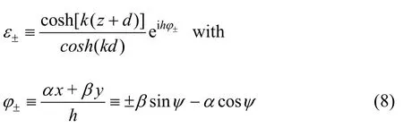
One has 1t≈ in deep water show that the Fourier variables and in Eq.(10) are defined in terms of the wave number kvia relations

The wavefunctionsε±defined by Eq.(8)and Eq.(10) correspond to plane waves that propagate at anglesγ±from the -axis given by

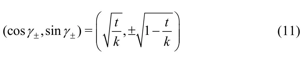
The dispersion relation Eq.(9) defines real plane waves if0()kdk≤where

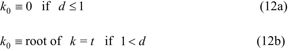
Thenon-dimensional velocity potentialφW≡ΦWg /V3associated with the waves created by the ship,the corresponding flow velocity≡and the elevation0)of the free surfaceabove or below theplane z = 0are given by related linear superpositions of the elementary wave function ε±(k,x)defined by Eq.(8).In particular,(x)is given by

where Remeans that the real part is considered, and thefiniteupper limit of integration k∞＜∞ filters unrealisticshort waves(notably wavesthat are influenced by surfacetension).The flow potential φWand the related flow velocitiesandare given by integral representations that aresimilar to Eq.(13),which isthen only considered herefor simplicity.

Theamplitude functions A±( k )in thewave integral Eq.(13) are defined in terms of distributions of elementary wave functions E±( k , ξ/ F r2)defined as

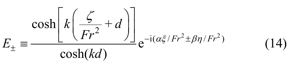
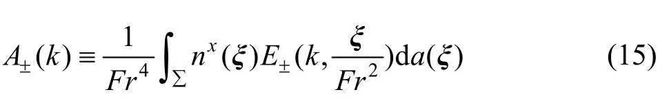
whereda(ξ)denotes the differential element of area at thepoint ξof ∑ ,and nx(ξ)is the x-component of the unit vector n(ξ) the normal to∑at ξand points outside the ship. The integration over theshiphull surface ∑in Eq.(15)is performed over the entire surface ∑to evaluate ship waves aft of the ship stern, but is only performed over the portion Fr2x≤ toevaluate near-field ship waves in the flow region x ≤ξ/Fr2located aft of the ship section x = ξ /Fr2.

2. Stationary phase and numerical evaluation

Accuratenumerical evaluation of thewave integral Eq.(13) is a critical element of the prediction of far-field and near-field ship waves, as was already noted.Thisimportant basicelement isa nontrivial task for large distances h ≡Hg/V2aft of theship because the trigonometric functionseihφ±in Eq.(13)oscillate very rapidly if 1?h.

Indeed,an ordinary integration rule (e.g.,Gaussian or Simpson)requires a hugenumber of integration points and is impractical for 1?h. The Filon numerical integration rule for rapidly oscillating integrands given in Ref.[18] is not well suited for case when points of stationary phase exist, as is the case for the wave integral Eq.(13), and moreover is not suited in the near field.

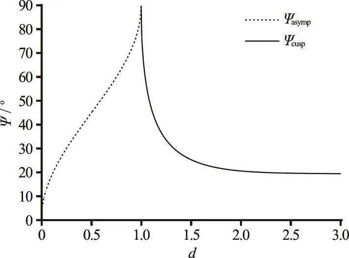
Fig.2 Asymptote angle for 0≤d≤1and cusp angle for 1≤d≤3

The method of stationary phasegiven in Kelvin[19]yields a simple analytical approximation to the wave integral Eq.(13) for 1?h. However, this classical far-field approximation is singular at the cusp anglesψ = ± ψcusp(d)if 1＜dor at theasymptote anglesψ = ± ψasymp(d)if d＜1, and is not valid in the vicinity of these important wake angles as well as for ψcusp＜|ψ |or ψasymp＜|ψ|,i.e.,outsidethe Kelvin-Havelock ship wake. The cusp and asymptote anglesψcusp(d)and ψasymp(d)aredepicted in Fig.2 and considered in Refs.[5-7].

However,theidea underlying themethod of stationary phase readily suggests a practical numerical method. This method, considered in Ref.[15], is now explained.As iswellknown,thebasic idea of Kelvin'sstationary-phaseapproximation isthat the dominant contribution to an integral of the form Eq.(2)with an integrant that involves a rapidly oscillatory trigonometric function

stems from points where phase is stationary, i.e.,from points where the derivativeφ′of vanishes.Thus,isφ′vanishes at a point =sφφwithin the range of integration, the function can be modified as

and σ2isa parameter that must be chosen judiciously. The analysis and numerical test that are required tochooseparameter in thefunction Eq.(17) are simple if the phase function only has distinct points of stationary phase whereφ′=0and φ′≠ 0 ,but aremorecomplicated for pointsof stationary phase where both φ′and φ′vanish,as is shown in Ref.[15]. An alternative to the modified function ?defined by Eq.(17) and used in Ref.[15]is considered here. The alternative modification of the trigonometric function that isconsidered hereis the function

and nisa parameter.Thealternativefunction Eq.(18) presumes that the points of stationary phase sφare known,as is the casefor ship waves.The parameter nin Eq.(18)controlsthe extent of the vicinity of the stationary pointsφwhereεε≈~and we take =4n in this paper.

Thefunction Eq.(16)can bemodified as in Eq.(17) or Eq.(18) without appreciably affecting the value of the integral Eq.(2). Indeed, the functions? and ~are nearly identical to the function in the vicinity φ ≈φsof a point of stationary phaseφ= φs,but one hasε??1and ε~?1outside the vicinity of thestationary point,i.e.,within theportion of the range of integration where the function oscillates rapidly and therefore does not contribute appreciably to the value of the integral Eq.(2). Specifically, Eq.(16)and Eq.(18) yield

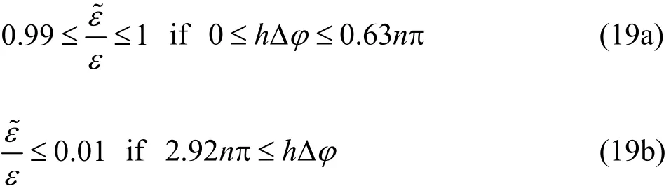
Thus, the function ~defined by Eq.(18) differs from the function defined by Eq.(16) less than 1% for h Δ φ≤0.63n π, decays smoothly for 0.63nπ ≤hΔφ≤2.92nπ,and isnegligibly small(and the rapid oscillations of the function are effectively damped)for 2.92nπ≤hΔ.

The numericalmethod considered hereis illustrated in Fig.3. This figure depicts the function ,themodified function ~and therelated function ε~/εfor a particular case associated with ship waves,considered in thenext section.Accuratenumerical integration via a common (Gaussian or Simpson)integration rule would require a very large number of integration points in the regions where the function oscillates rapidly, even though their contributions are insignificant.The function ~is nearly nil in these regions. A (wide) integration step that is adapted to the (slow) variation of the function in the vicinity of thepoint of stationary phase,where varies slowly, can then also be used in the region where oscillates rapidly.

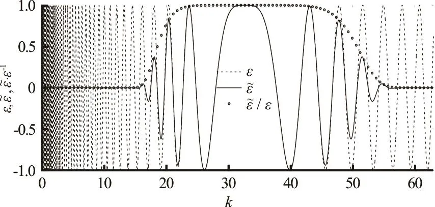
Fig.3 Functions,ε~and /εε~for a particular case associated with ship waves

3. Ship waves in calm water of f1inite depth

The numerical method explained in the previous section is now applied to the wave integral Eq.(13)associated with ship waves in calm water of uniform finite depth.

TherelationsEq.(10)show that thephase function defined by Eq.(8) and its first and second derivatives are given by

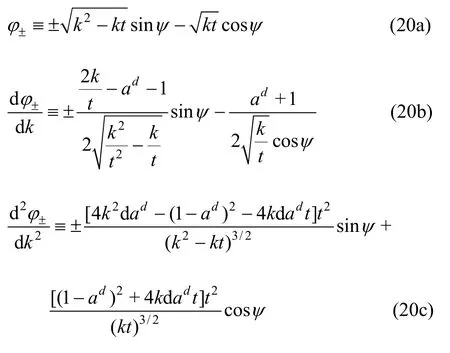
where adis defined as

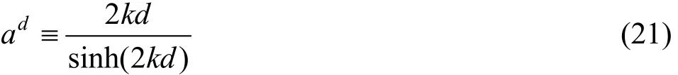
The points of stationary phase are determined by the roots of d/d=0kφ±, i.e.

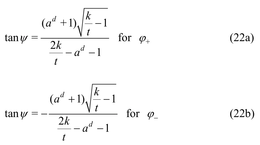
Equation (22)havenorealsolution for ray angles-π / 2 ≤ ψ ≤ 0 or 0≤ ψ ≤ π / 2,respectively.Only waves that correspond to0 ≤ ψ ≤ π /2, i.e., waves in the positive half 0≤y, are considered hereafter due to symmetry about the axis y = 0.

Figure 4 depicts the derivatives(,)kφψ′of the phasefunction (,)kφψfor four ray anglesand twowater depthsd.Thisfigureillustrateswellknown basic properties of ship waves in finite water depth,considered in Refs.[6,7],and therelated derivative φ′of the phase function .

Fig.4 Variations of the derivatives(,)kφψ′of the phase function (,)kφψwithin the range 010k≤≤at Froude number =0.4Fr and two water different depths

For water depth d ＜ 1 , no transverse waves exist and divergent waves exist for ray anglesψ ≤ψasymp,i.e., inside the asymptoteψ =ψasympof the Kelvin-Havelock wake,whereas for 1＜d,transverse and divergent wavesexist inside thecuspψ =ψcuspof the Kelvin-Havelock wake. These basic properties are illustrated in Fig.4.Specifically,for a water depth d =0.625, the left side of the figure shows that φ′increases monotonically for 0≤kand vanishes at a point k = kDfor ray anglesψ ≤ψ ≈52.23o.

asympThe point of stationary phase k = kDonly exists for ψ≤and corresponds to divergent waves. The right side of Fig.4, which corresponds to a water depth d =1.25,showsthat φ′vanishesat twodistinct pointsk = kTand k = kDfor ray angles ψ≤ψcusp≈33.74o.The twopointsof stationary phase k = kTand k = kD,which correspond to transverseand divergent waves,only exist for ψ≤ψcuspand coalescefor ψ=ψcusp,whereone then has kT= kD=kC.

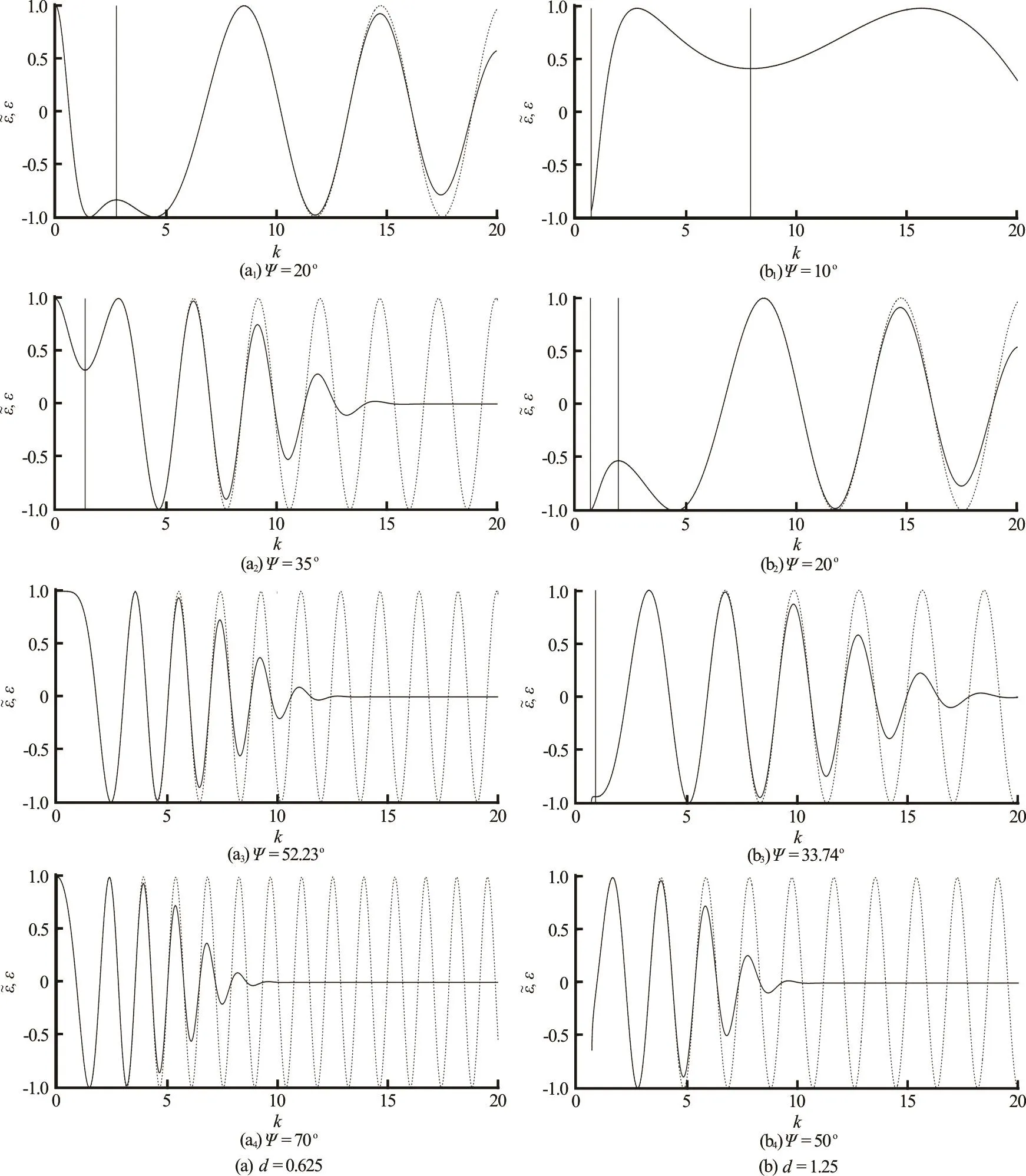
Fig.5 Real part of the trigonometric function and the related modified function ε~defined by Eq.(16) and Eq.(17) for two water depths at =5h along four ray angles

The term Δ φ≡ φ- φsin expression Eq.(18) for the function ~is then given by

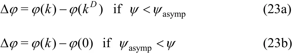
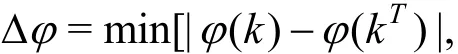
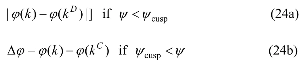
if 1d＜ , or if d＜ 1 .Thepointsof stationary phase kDin Eq.(23),kTand kDin Eq.(24) and kCin Eq.(24)arerootsof thestationary-phaserelation φ′=0 whereφ′isgiven by Eq.(20).These roots,the asymptoteangle ψasympin Eq.(23),and thecusp angle ψcuspin Eq.(24) are further considered in the literature[5-7].

Applications of thenumericalmethod are illustrated in Fig.5and for water depth d =0.625 and d =1.25. Wave patterns are also shown in Fig.6.

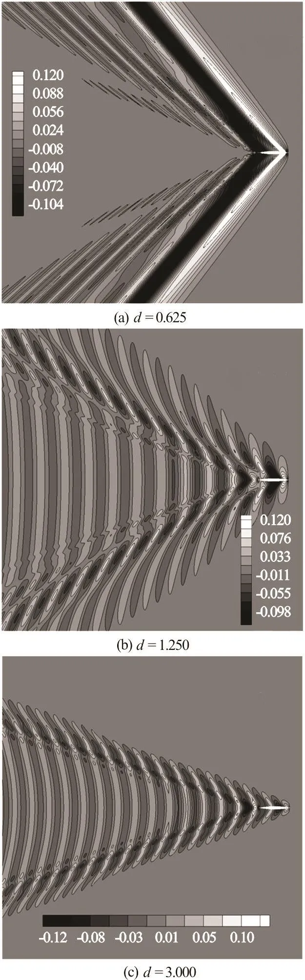
Fig.6 Ship waves created by the Wigley hull at Froude number Fr = 0.3in three water depths

4. Conclusions

The practical numerical method-inspired by the method of stationary phase-for evaluating the Fourier integral that defines far-field and near-field ship wavesgiven in Ref.[15]for deepwater hasbeen extended to the more general case of shallow water,and modified. The modification given here, based on an explicit use of the dispersion relation to determine the points of stationary phase, yields a method that is simpler,aswellasmoregeneral,than themethod previously given in Ref.[15].

The method given in Ref.[15] for ship waves in deep water and the related method given here for ship waves in uniform finite water depth can be applied more generally toa broad class of integrals, of the form Eq.(2), that involve a rapidly oscillatory trigonometric function with a phasefunction whose first derivative (and possibly also higher derivatives, as is the case for ship waves) vanishes at one or several points (commonly called points of stationary phase)within the range of integration.

[1]Havelock T. H. The propagation of groups of waves in dispersivemedia,with applicationstowaves on water produced by a traveling disturbance [C]. Proceedings of the Royal Society of London. London, UK, 1908, 81(549):398-430.

[2]Kinoshita M. Wave resistance of a sphere in a shallow sea[J]. Journal of Zosen Kiokai, 2009, 1951: 19-38.

[3]Wehausen J. V., Laitone E. V. Surface waves [M]. Berlin,Heidelberg, Germany: Springer, 1960, 9: 446-778.

[4]Chen X., ZhaoR.Steady free-surfaceflow in water of finite depth [C].16th International Workshop onWater Waves and Floating Bodies. Hiroshima, Japan, 2001.

[5]Noblesse F., Yang C. Elementary water waves [J]. Journal of Engineering Mathematics, 2007, 59(3): 277-299.

[6]Zhu Y., He J., Zhang C. et al. Farfield waves created by a monohull ship in shallow water [J]. European Journal of Mechanics-B/Fluids, 2015, 49: 226-34.

[7]Zhu Y., Ma C., Wu H. et al. Farfield waves created by a catamaran in shallow water [J].EuropeanJournal of Mechanics-B/Fluids, 2016, 59: 197-204.

[8]Noblesse F., Huang F., Yang C. The Neumann–Michell theory of ship waves [J]. Journal of Engineering Mathematics, 2013, 79(1): 51-71.

[9]Huang F., Yang C., Noblesse F. Numerical implementation and validation of the Neumann–Michell theory of ship waves [J]. European Journal of Mechanics-B/Fluids,2013, 42: 47-68.

[10] Ma C., Zhang C., Chen X. et al. Practical estimation of sinkage and trim for common generic monohull ships [J].Ocean Engineering, 2016, 126: 203-16.

[11] Ma C., Zhang C., Huang F. et al. Practical evaluation of sinkage and trim effects on the drag of a common generic freely floating monohull ship [J]. Applied Ocean Research,2017, 65: 1-11.

[12] Zhang C., Zhu Y., Wu H. et al. Practical numerical evaluation of far-field and near-field ship waves in shallow water[C].32nd International Workshop on Water Wavesand Floating Bodies. Dalian, China, 2017, 225-228.

[13]NoblesseF.Alternative integral representationsfor the Green function of the theory of ship wave resistance [J].Journal of Engineering Mathematics, 1981, 15(4): 241-65.

[14] Noblesse F., Huang F., Yang C. Evaluation of ship waves at thefree surface and removalof short waves[J].EuropeanJournal of Mechanics-B/Fluids,2013,38:22-37.

[15] Zhang C., He J., Zhu Y. et al. Stationary phase and numerical evaluation of far-field and near-field ship waves [J].EuropeanJournal of Mechanics-B/Fluids,2015,52:28-37.

[16]Noblesse F.,Delhommeau G.,Liu H.et al.Shipbow waves[J].Journal of Hydrodynamics,2013,25(4):491-500.

[17] Hogner E. Hydromech [C]. Hydromechanische Probleme des Schiffsantriebs. Hamburg, Germany, 1932, 99-114.

[18]Filon L. N.On a quadrature formula for trigonometric integrals[C].Proceedings of the Royal Society of Edinburgh. Edinburgh, UK, 1930, 49: 38-47.

[19] Kelvin W. T. Popular lectures and addresses: Navigational affairs [M]. London, UK: Macmillan and Company, 1891.

June 6, 2017, Revised July 31, 2017)

* Biography: Chen-liang Zhang (1990-), Male,Master, Engineer